Matlab散点密度图

slandarer 2022-05-23 我要评论

效果

原理也很简单，通过matlab自带的ksdensity获得网格每一点密度，通过密度拟合曲面，再计算每个数据点对应的概率，并将概率映射到颜色即可
为了怕大家找不到函数这次工具函数放到最前面

1工具函数完整代码

function [CData,h,XMesh,YMesh,ZMesh,colorList]=density2C(X,Y,XList,YList,colorList)
[XMesh,YMesh]=meshgrid(XList,YList);
XYi=[XMesh(:) YMesh(:)];
F=ksdensity([X,Y],XYi);
ZMesh=zeros(size(XMesh));
ZMesh(1:length(F))=F;

h=interp2(XMesh,YMesh,ZMesh,X,Y);
if nargin<5
colorList=[0.2700         0    0.3300
    0.2700    0.2300    0.5100
    0.1900    0.4100    0.5600
    0.1200    0.5600    0.5500
    0.2100    0.7200    0.4700
    0.5600    0.8400    0.2700
    0.9900    0.9100    0.1300];
end
colorFunc=colorFuncFactory(colorList);
CData=colorFunc((h-min(h))./(max(h)-min(h)));
colorList=colorFunc(linspace(0,1,100)');

function colorFunc=colorFuncFactory(colorList)
x=(0:size(colorList,1)-1)./(size(colorList,1)-1);
y1=colorList(:,1);y2=colorList(:,2);y3=colorList(:,3);
colorFunc=@(X)[interp1(x,y1,X,'pchip'),interp1(x,y2,X,'pchip'),interp1(x,y3,X,'pchip')];
end
end

2参数说明

输入：

X,Y 散点坐标
XList,YList 用来构造密度曲面网格的序列，其实就是把XLim，YLim分成小份，例如XList=0:0.1:10
colorList 颜色表mx3数组，用来构造将高度映射到颜色函数的数据表

输出：

CData各个点对应颜色
h 各个点对应核密度
XMesh,YMesh,ZMesh 核密度曲面数据
colorList 插值后更细密的颜色表

3使用方式

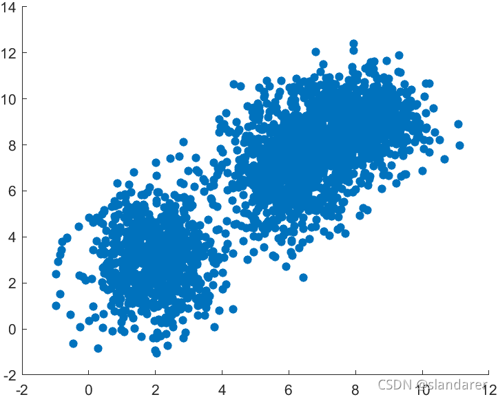
假如编写了如下程序：

PntSet1=mvnrnd([2 3],[1 0;0 2],800);
PntSet2=mvnrnd([6 7],[1 0;0 2],800);
PntSet3=mvnrnd([8 9],[1 0;0 1],800);

PntSet=[PntSet1;PntSet2;PntSet3];
scatter(PntSet(:,1),PntSet(:,2),'filled');

结果：

3.1散点赋色

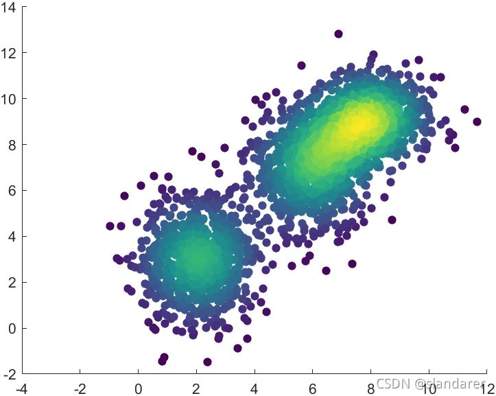
将上面那段代码改写

PntSet1=mvnrnd([2 3],[1 0;0 2],800);
PntSet2=mvnrnd([6 7],[1 0;0 2],800);
PntSet3=mvnrnd([8 9],[1 0;0 1],800);

PntSet=[PntSet1;PntSet2;PntSet3];

CData=density2C(PntSet(:,1),PntSet(:,2),-2:0.1:15,-2:0.1:15);
scatter(PntSet(:,1),PntSet(:,2),'filled','CData',CData);

3.2等高线图

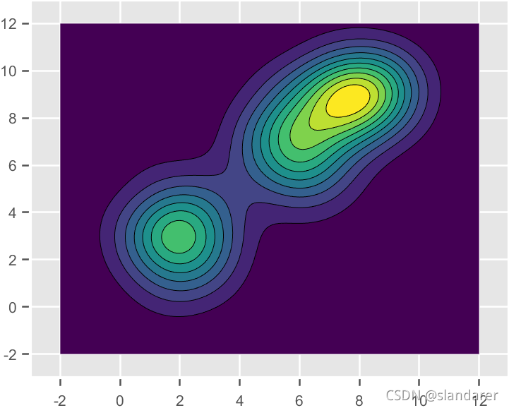
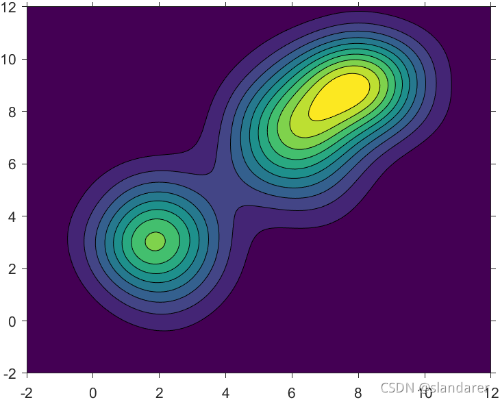
PntSet1=mvnrnd([2 3],[1 0;0 2],800);
PntSet2=mvnrnd([6 7],[1 0;0 2],800);
PntSet3=mvnrnd([8 9],[1 0;0 1],800);

PntSet=[PntSet1;PntSet2;PntSet3];


[~,~,XMesh,YMesh,ZMesh,colorList]=density2C(PntSet(:,1),PntSet(:,2),-2:0.1:12,-2:0.1:12);
colormap(colorList)
contourf(XMesh,YMesh,ZMesh,10)

3.3带直方图的散点图

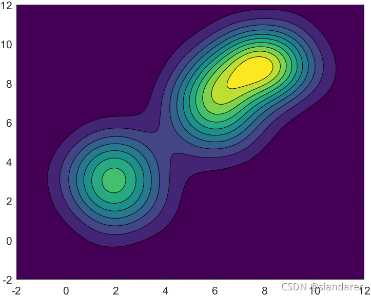
PntSet1=mvnrnd([2 3],[1 0;0 2],800);
PntSet2=mvnrnd([6 7],[1 0;0 2],800);
PntSet3=mvnrnd([8 9],[1 0;0 1],800);

PntSet=[PntSet1;PntSet2;PntSet3];

colorList=[0.9400    0.9700    0.9600
    0.8900    0.9300    0.9200
    0.8200    0.9100    0.8800
    0.6900    0.8500    0.7700
    0.5900    0.7800    0.6900
    0.5500    0.7500    0.6500
    0.4500    0.6500    0.5600
    0.4000    0.5800    0.4900
    0.3500    0.5100    0.4200
    0.2500    0.3600    0.3100
    0.1300    0.1700    0.1400];
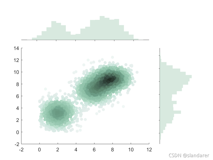
CData=density2C(PntSet(:,1),PntSet(:,2),-2:0.1:15,-2:0.1:15,colorList);

set(gcf,'Color',[1 1 1]);

% 主分布图
ax1=axes('Parent',gcf);hold(ax1,'on')
scatter(ax1,PntSet(:,1),PntSet(:,2),'filled','CData',CData);
ax1.Position=[0.1,0.1,0.6,0.6];

% X轴直方图
ax2=axes('Parent',gcf);hold(ax2,'on')
histogram(ax2,PntSet(:,1),'FaceColor',[0.78 0.88 0.82],...
    'EdgeColor','none','FaceAlpha',0.7)
ax2.Position=[0.1,0.75,0.6,0.15];
ax2.YColor='none';
ax2.XTickLabel='';
ax2.TickDir='out';
ax2.XLim=ax1.XLim;

% Y轴直方图
ax3=axes('Parent',gcf);hold(ax3,'on')
histogram(ax3,PntSet(:,2),'FaceColor',[0.78 0.88 0.82],...
    'EdgeColor','none','FaceAlpha',0.7,'Orientation','horizontal')
ax3.Position=[0.75,0.1,0.15,0.6];
ax3.XColor='none';
ax3.YTickLabel='';
ax3.TickDir='out';
ax3.YLim=ax1.YLim;

3.4带直方图的等高线图

PntSet1=mvnrnd([2 3],[1 0;0 2],800);
PntSet2=mvnrnd([6 7],[1 0;0 2],800);
PntSet3=mvnrnd([8 9],[1 0;0 1],800);

PntSet=[PntSet1;PntSet2;PntSet3];
colorList=[0.9300    0.9500    0.9700
    0.7900    0.8400    0.9100
    0.6500    0.7300    0.8500
    0.5100    0.6200    0.7900
    0.3700    0.5100    0.7300
    0.2700    0.4100    0.6300
    0.2100    0.3200    0.4900
    0.1500    0.2200    0.3500
    0.0900    0.1300    0.2100
    0.0300    0.0400    0.0700];
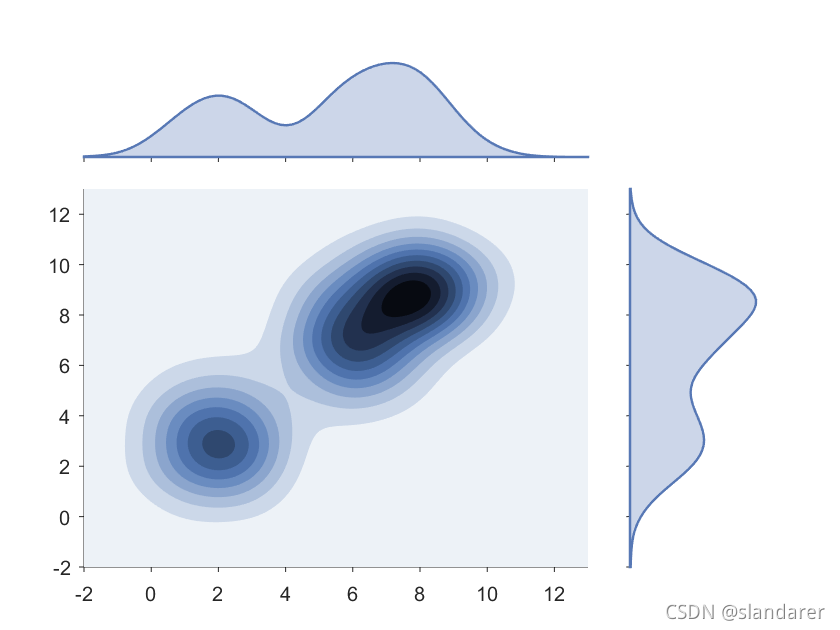
[~,~,XMesh,YMesh,ZMesh,colorList]=density2C(PntSet(:,1),PntSet(:,2),-2:0.1:13,-2:0.1:13,colorList);


set(gcf,'Color',[1 1 1]);
% 主分布图
ax1=axes('Parent',gcf);hold(ax1,'on')
colormap(colorList)
contourf(XMesh,YMesh,ZMesh,10,'EdgeColor','none')
ax1.Position=[0.1,0.1,0.6,0.6];
ax1.TickDir='out';

% X轴直方图
ax2=axes('Parent',gcf);hold(ax2,'on')
[f,xi]=ksdensity(PntSet(:,1));
fill([xi,xi(1)],[f,0],[0.34 0.47 0.71],'FaceAlpha',...
    0.3,'EdgeColor',[0.34 0.47 0.71],'LineWidth',1.2)
ax2.Position=[0.1,0.75,0.6,0.15];
ax2.YColor='none';
ax2.XTickLabel='';
ax2.TickDir='out';
ax2.XLim=ax1.XLim;

% Y轴直方图
ax3=axes('Parent',gcf);hold(ax3,'on')
[f,yi]=ksdensity(PntSet(:,2));
fill([f,0],[yi,yi(1)],[0.34 0.47 0.71],'FaceAlpha',...
    0.3,'EdgeColor',[0.34 0.47 0.71],'LineWidth',1.2)
ax3.Position=[0.75,0.1,0.15,0.6];
ax3.XColor='none';
ax3.YTickLabel='';
ax3.TickDir='out';
ax3.YLim=ax1.YLim;

4使用方式扩展–与ggplot修饰器联动

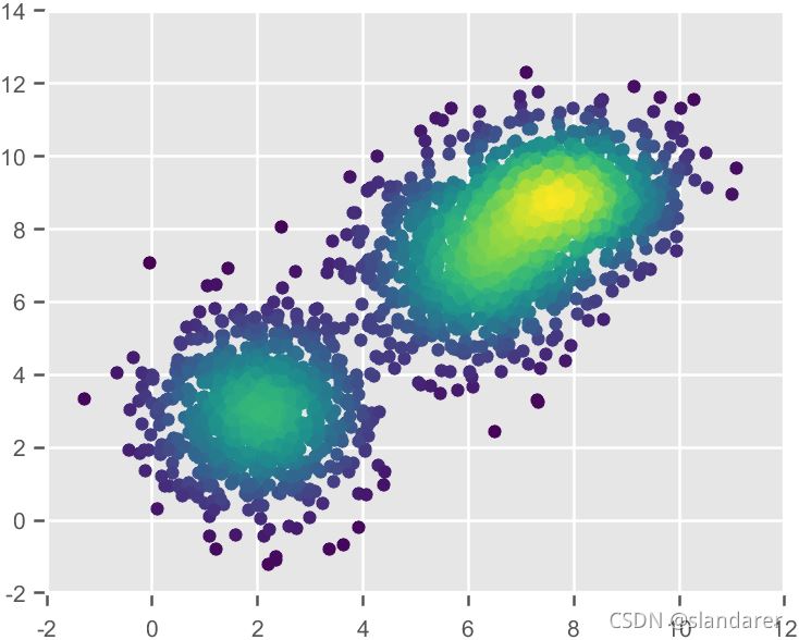
ggplot风格修饰器：(点击图片跳转链接)

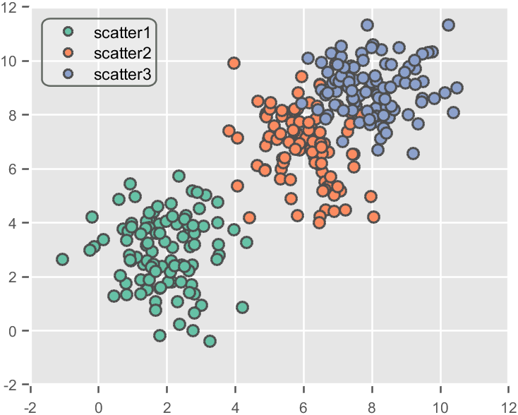
示例1

PntSet1=mvnrnd([2 3],[1 0;0 2],800);
PntSet2=mvnrnd([6 7],[1 0;0 2],800);
PntSet3=mvnrnd([8 9],[1 0;0 1],800);

PntSet=[PntSet1;PntSet2;PntSet3];

ax=gca;
ax.XLim=[-1 13];
ax.YLim=[-1 13];
ax=ggplotAxes2D(ax);

CData=density2C(PntSet(:,1),PntSet(:,2),0:0.1:15,0:0.1:15);
scatter(PntSet(:,1),PntSet(:,2),'filled','CData',CData);

是不是瞬间有那味了：

示例2

PntSet1=mvnrnd([2 3],[1 0;0 2],800);
PntSet2=mvnrnd([6 7],[1 0;0 2],800);
PntSet3=mvnrnd([8 9],[1 0;0 1],800);

PntSet=[PntSet1;PntSet2;PntSet3];

ax=gca;
ax.XLim=[-3 13];
ax.YLim=[-3 13];
ax=ggplotAxes2D(ax);

[~,~,XMesh,YMesh,ZMesh,colorList]=density2C(PntSet(:,1),PntSet(:,2),-2:0.1:12,-2:0.1:12);
colormap(colorList)
contourf(XMesh,YMesh,ZMesh,10)

Matlab散点密度图

效果

1工具函数完整代码

2参数说明

3使用方式

3.1散点赋色

3.2等高线图

3.3带直方图的散点图

3.4带直方图的等高线图

4使用方式扩展–与ggplot修饰器联动

相关文章

猜您喜欢

今日热门