在pytorch中想自定义求导函数,通过实现torch.autograd.Function并重写forward和backward函数,来定义自己的自动求导运算。参考官网上的demo:传送门
直接上代码,定义一个ReLu来实现自动求导
import torch

class MyRelu(torch.autograd.Function):
    @staticmethod
    def forward(ctx, input):
        # 我们使用ctx上下文对象来缓存,以便在反向传播中使用,ctx存储时候只能存tensor
        # 在正向传播中,我们接收一个上下文对象ctx和一个包含输入的张量input;
        # 我们必须返回一个包含输出的张量,
        # input.clamp(min = 0)表示讲输入中所有值范围规定到0到正无穷,如input=[-1,-2,3]则被转换成input=[0,0,3]
        ctx.save_for_backward(input)

        # 返回几个值,backward接受参数则包含ctx和这几个值
        return input.clamp(min = 0)

    @staticmethod
    def backward(ctx, grad_output):
        # 把ctx中存储的input张量读取出来
        input, = ctx.saved_tensors

        # grad_output存放反向传播过程中的梯度
        grad_input = grad_output.clone()

        # 这儿就是ReLu的规则,表示原始数据小于0,则relu为0,因此对应索引的梯度都置为0
        grad_input[input < 0] = 0
        return grad_input
进行输入数据并测试
dtype = torch.float
device = torch.device('cuda' if torch.cuda.is_available() else 'cpu')
# 使用torch的generator定义随机数,注意产生的是cpu随机数还是gpu随机数
generator=torch.Generator(device).manual_seed(42)

# N是Batch, H is hidden dimension,
# D_in is input dimension;D_out is output dimension.
N, D_in, H, D_out = 64, 1000, 100, 10

x = torch.randn(N, D_in, device=device, dtype=dtype,generator=generator)
y = torch.randn(N, D_out, device=device, dtype=dtype, generator=generator)

w1 = torch.randn(D_in, H, device=device, dtype=dtype, requires_grad=True, generator=generator)
w2 = torch.randn(H, D_out, device=device, dtype=dtype, requires_grad=True, generator=generator)

learning_rate = 1e-6
for t in range(500):
    relu = MyRelu.apply
    # 使用函数传入参数运算
    y_pred = relu(x.mm(w1)).mm(w2)
	# 计算损失
    loss = (y_pred - y).pow(2).sum()
    if t % 100 == 99:
        print(t, loss.item())
    # 传播
    loss.backward()
    with torch.no_grad():
        w1 -= learning_rate * w1.grad
        w2 -= learning_rate * w2.grad

        w1.grad.zero_()
        w2.grad.zero_()
retain_graph设为True,可以进行两次反向传播


import torch
import torch.nn as nn
import matplotlib.pyplot as plt
import numpy as np
torch.manual_seed(10)
#========生成数据=============
sample_nums = 100
mean_value = 1.7
bias = 1
n_data = torch.ones(sample_nums,2)
x0 = torch.normal(mean_value*n_data,1)+bias#类别0数据
y0 = torch.zeros(sample_nums)#类别0标签
x1 = torch.normal(-mean_value*n_data,1)+bias#类别1数据
y1 = torch.ones(sample_nums)#类别1标签
train_x = torch.cat((x0,x1),0)
train_y = torch.cat((y0,y1),0)
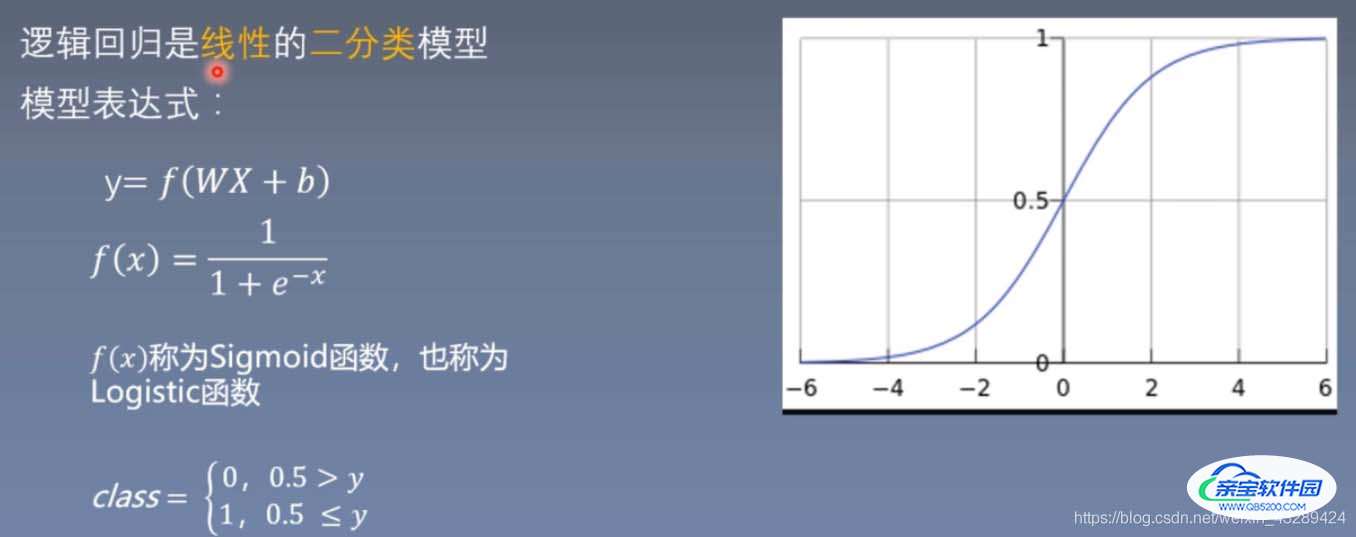
#==========选择模型===========
class LR(nn.Module):
def __init__(self):
super(LR,self).__init__()
self.features = nn.Linear(2,1)
self.sigmoid = nn.Sigmoid()
def forward(self,x):
x = self.features(x)
x = self.sigmoid(x)
return x
lr_net = LR()#实例化逻辑回归模型
#==============选择损失函数===============
loss_fn = nn.BCELoss()
#==============选择优化器=================
lr = 0.01
optimizer = torch.optim.SGD(lr_net.parameters(),lr = lr,momentum=0.9)
#===============模型训练==================
for iteration in range(1000):
#前向传播
y_pred = lr_net(train_x)#模型的输出
#计算loss
loss = loss_fn(y_pred.squeeze(),train_y)
#反向传播
loss.backward()
#更新参数
optimizer.step()
#绘图
if iteration % 20 == 0:
mask = y_pred.ge(0.5).float().squeeze() #以0.5分类
correct = (mask==train_y).sum()#正确预测样本数
acc = correct.item()/train_y.size(0)#分类准确率
plt.scatter(x0.data.numpy()[:,0],x0.data.numpy()[:,1],c='r',label='class0')
plt.scatter(x1.data.numpy()[:,0],x1.data.numpy()[:,1],c='b',label='class1')
w0,w1 = lr_net.features.weight[0]
w0,w1 = float(w0.item()),float(w1.item())
plot_b = float(lr_net.features.bias[0].item())
plot_x = np.arange(-6,6,0.1)
plot_y = (-w0*plot_x-plot_b)/w1
plt.xlim(-5,7)
plt.ylim(-7,7)
plt.plot(plot_x,plot_y)
plt.text(-5,5,'Loss=%.4f'%loss.data.numpy(),fontdict={'size':20,'color':'red'})
plt.title('Iteration:{}\nw0:{:.2f} w1:{:.2f} b{:.2f} accuracy:{:2%}'.format(iteration,w0,w1,plot_b,acc))
plt.legend()
plt.show()
plt.pause(0.5)
if acc > 0.99:
break以上为个人经验,希望能给大家一个参考,也希望大家多多支持。