from scipy.interpolate import interp1d
1维插值算法
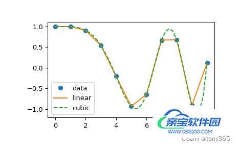
from scipy.interpolate import interp1d
x = np.linspace(0, 10, num=11, endpoint=True)
y = np.cos(-x**2/9.0)
f = interp1d(x, y)
f2 = interp1d(x, y, kind='cubic')
xnew = np.linspace(0, 10, num=41, endpoint=True)
import matplotlib.pyplot as plt
plt.plot(x, y, 'o', xnew, f(xnew), '-', xnew, f2(xnew), '--')
plt.legend(['data', 'linear', 'cubic'], loc='best')
plt.show()
数据点,线性插值结果,cubic插值结果:
from scipy.interpolate import interp2d
from scipy.interpolate import griddata
多为插值方法,可以应用在2Dlut,3Dlut的生成上面,比如当我们已经有了两组RGB映射数据, 可以插值得到一个查找表。
二维插值的例子如下:
import numpy as np
from scipy import interpolate
import matplotlib.pyplot as plt
from scipy.interpolate import griddata, RegularGridInterpolator, Rbf
if __name__ == "__main__":
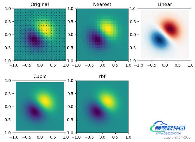
x_edges, y_edges = np.mgrid[-1:1:21j, -1:1:21j]
x = x_edges[:-1, :-1] + np.diff(x_edges[:2, 0])[0] / 2.
y = y_edges[:-1, :-1] + np.diff(y_edges[0, :2])[0] / 2.
# x_edges, y_edges 是 20个格的边缘的坐标, 尺寸 21 * 21
# x, y 是 20个格的中心的坐标, 尺寸 20 * 20
z = (x + y) * np.exp(-6.0 * (x * x + y * y))
print(x_edges.shape, x.shape, z.shape)
plt.figure()
lims = dict(cmap='RdBu_r', vmin=-0.25, vmax=0.25)
plt.pcolormesh(x_edges, y_edges, z, shading='flat', **lims) # plt.pcolormesh(), plt.colorbar() 画图
plt.colorbar()
plt.title("Sparsely sampled function.")
plt.show()
# 使用grid data
xnew_edges, ynew_edges = np.mgrid[-1:1:71j, -1:1:71j]
xnew = xnew_edges[:-1, :-1] + np.diff(xnew_edges[:2, 0])[0] / 2. # xnew其实是 height new
ynew = ynew_edges[:-1, :-1] + np.diff(ynew_edges[0, :2])[0] / 2.
grid_x, grid_y = xnew, ynew
print(x.shape, y.shape, z.shape)
points = np.hstack((x.reshape(-1, 1), y.reshape(-1, 1)))
z1 = z.reshape(-1, 1)
grid_z0 = griddata(points, z1, (grid_x, grid_y), method='nearest').squeeze()
grid_z1 = griddata(points, z1, (grid_x, grid_y), method='linear').squeeze()
grid_z2 = griddata(points, z1, (grid_x, grid_y), method='cubic').squeeze()
rbf = Rbf(points[:, 0], points[:, 1], z, epsilon=2)
grid_z3 = rbf(grid_x, grid_y)
plt.subplot(231)
plt.imshow(z.T, extent=(-1, 1, -1, 1), origin='lower')
plt.plot(points[:, 0], points[:, 1], 'k.', ms=1)
plt.title('Original')
plt.subplot(232)
plt.imshow(grid_z0.T, extent=(-1, 1, -1, 1), origin='lower')
plt.title('Nearest')
plt.subplot(233)
plt.imshow(grid_z1.T, extent=(-1, 1, -1, 1), origin='lower', cmap='RdBu_r')
plt.title('Linear')
plt.subplot(234)
plt.imshow(grid_z2.T, extent=(-1, 1, -1, 1), origin='lower')
plt.title('Cubic')
plt.subplot(235)
plt.imshow(grid_z3.T, extent=(-1, 1, -1, 1), origin='lower')
plt.title('rbf')
plt.gcf().set_size_inches(8, 6)
plt.show()
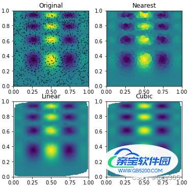
示例2:
def func(x, y):
    return x*(1-x)*np.cos(4*np.pi*x) * np.sin(4*np.pi*y**2)**2


grid_x, grid_y = np.mgrid[0:1:100j, 0:1:200j]


rng = np.random.default_rng()
points = rng.random((1000, 2))
values = func(points[:,0], points[:,1])

from scipy.interpolate import griddata
grid_z0 = griddata(points, values, (grid_x, grid_y), method='nearest')
grid_z1 = griddata(points, values, (grid_x, grid_y), method='linear')
grid_z2 = griddata(points, values, (grid_x, grid_y), method='cubic')

import matplotlib.pyplot as plt
plt.subplot(221)
plt.imshow(func(grid_x, grid_y).T, extent=(0,1,0,1), origin='lower')
plt.plot(points[:,0], points[:,1], 'k.', ms=1)
plt.title('Original')
plt.subplot(222)
plt.imshow(grid_z0.T, extent=(0,1,0,1), origin='lower')
plt.title('Nearest')
plt.subplot(223)
plt.imshow(grid_z1.T, extent=(0,1,0,1), origin='lower')
plt.title('Linear')
plt.subplot(224)
plt.imshow(grid_z2.T, extent=(0,1,0,1), origin='lower')
plt.title('Cubic')
plt.gcf().set_size_inches(6, 6)
plt.show()
from scipy.interpolate import RegularGridInterpolator
已知一些grid上的值。
可以应用在2Dlut,3Dlut,当我们已经有了一个多维查找表,然后整个图像作为输入,得到查找和插值后的输出。
二维网格插值方法(好像和resize的功能比较一致)
# 使用RegularGridInterpolator
import matplotlib.pyplot as plt
from scipy.interpolate import RegularGridInterpolator

def F(u, v):
    return u * np.cos(u * v) + v * np.sin(u * v)

fit_points = [np.linspace(0, 3, 8), np.linspace(0, 3, 8)]
values = F(*np.meshgrid(*fit_points, indexing='ij'))

ut, vt = np.meshgrid(np.linspace(0, 3, 80), np.linspace(0, 3, 80), indexing='ij')
true_values = F(ut, vt)
test_points = np.array([ut.ravel(), vt.ravel()]).T

interp = RegularGridInterpolator(fit_points, values)
fig, axes = plt.subplots(2, 3, figsize=(10, 6))
axes = axes.ravel()
fig_index = 0
for method in ['linear', 'nearest', 'linear', 'cubic', 'quintic']:
    im = interp(test_points, method=method).reshape(80, 80)
    axes[fig_index].imshow(im)
    axes[fig_index].set_title(method)
    axes[fig_index].axis("off")
    fig_index += 1
axes[fig_index].imshow(true_values)
axes[fig_index].set_title("True values")
fig.tight_layout()
fig.show()
plt.show()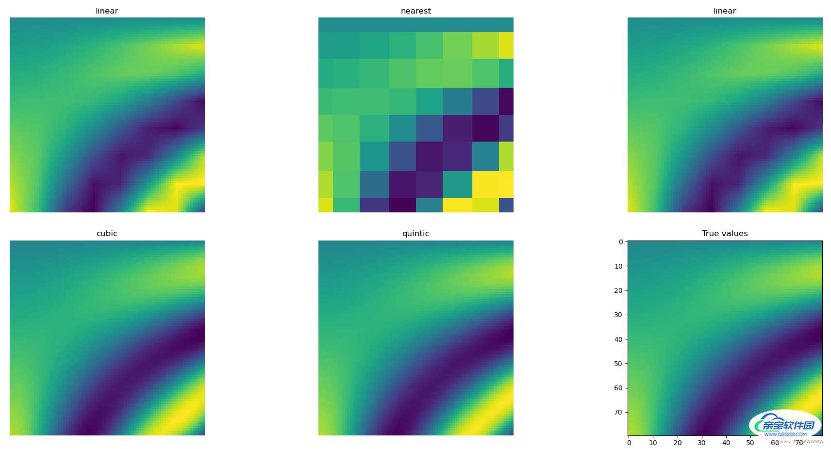
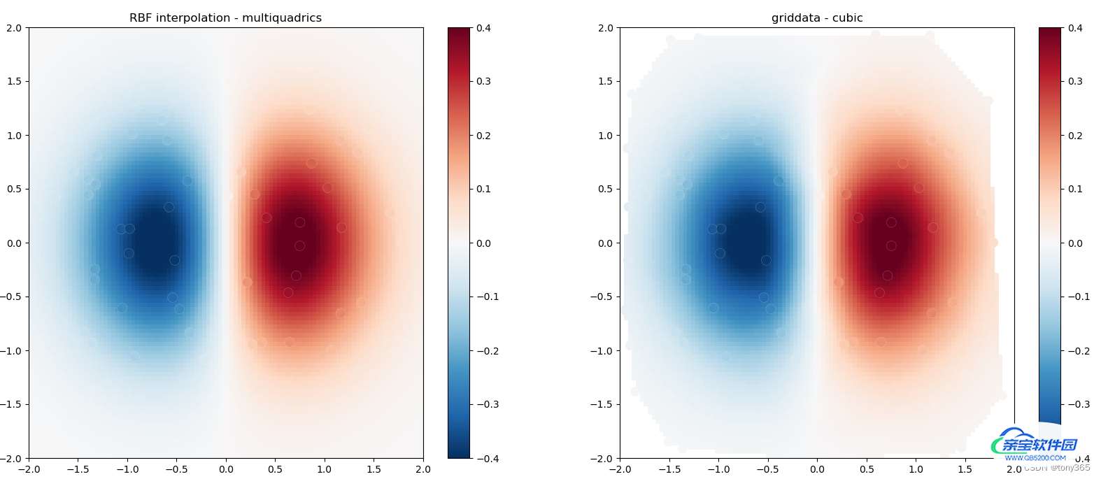
interpolate scattered 2-D data
import numpy as np
from scipy.interpolate import Rbf
import matplotlib.pyplot as plt
from matplotlib import cm

# 2-d tests - setup scattered data
rng = np.random.default_rng()
x = rng.random(100) * 4.0 - 2.0
y = rng.random(100) * 4.0 - 2.0
z = x * np.exp(-x ** 2 - y ** 2)


edges = np.linspace(-2.0, 2.0, 101)
centers = edges[:-1] + np.diff(edges[:2])[0] / 2.

XI, YI = np.meshgrid(centers, centers)
# use RBF
rbf = Rbf(x, y, z, epsilon=2)
Z1 = rbf(XI, YI)

points = np.hstack((x.reshape(-1, 1), y.reshape(-1, 1)))
Z2 = griddata(points, z, (XI, YI), method='cubic').squeeze()

# plot the result
plt.figure(figsize=(20,8))
plt.subplot(1, 2, 1)
X_edges, Y_edges = np.meshgrid(edges, edges)
lims = dict(cmap='RdBu_r', vmin=-0.4, vmax=0.4)
plt.pcolormesh(X_edges, Y_edges, Z1, shading='flat', **lims)
plt.scatter(x, y, 100, z, edgecolor='w', lw=0.1, **lims)
plt.title('RBF interpolation - multiquadrics')
plt.xlim(-2, 2)
plt.ylim(-2, 2)
plt.colorbar()

plt.subplot(1, 2, 2)
X_edges, Y_edges = np.meshgrid(edges, edges)
lims = dict(cmap='RdBu_r', vmin=-0.4, vmax=0.4)
plt.pcolormesh(X_edges, Y_edges, Z2, shading='flat', **lims)
plt.scatter(x, y, 100, z, edgecolor='w', lw=0.1, **lims)
plt.title('griddata - cubic')
plt.xlim(-2, 2)
plt.ylim(-2, 2)
plt.colorbar()
plt.show()
得到结果如下, RBF一定程度上和 griddata可以互用, griddata方法比较通用
[1]https://docs.scipy.org/doc/scipy/tutorial/interpolate.html