本篇是在之前两篇基础上接着写的:
吴恩达deepLearning.ai循环神经网络RNN学习笔记(理论篇)
从头构建循环神经网络RNN的向前传播(rnn in pure python)
也可以不看,如果以下有看不懂的,再回过头来看上面两篇也行。
前言
目录
-
阀门和状态描述
-
LSTM cell
-
LSTM整个过程
需要理解:
-
遗忘门,更新门,输出门的作用是什么,它们是怎么发挥作用的。
-
单元状态 cell state 是如何来选择性保留信息。
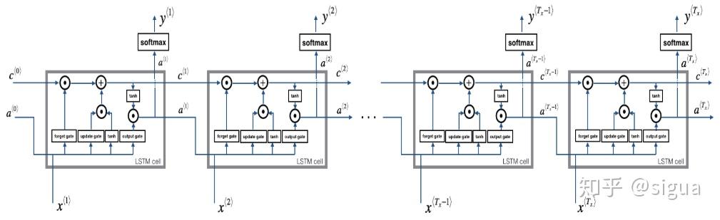
下面这张图将示意LSTM的操作。
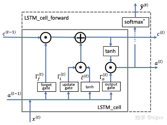
LSTM单元,它在每一个时间步长跟踪更新“单元状态”或者是记忆变量。
同之前讲的RNN例子一样,我们将以一个时间步长的LSTM单元执行开始,接着你就可以用for循环处理Tx个时间步长。
阀门和状态概述
遗忘门
概念:
-
假设我们正在阅读一段文本中的单词,并计划使用LSTM跟踪语法结构,例如判断主体是单数(“ puppy”)还是复数(“ puppies”)。
-
如果主体更改其状态(从单数词更改为复数词),那么先前的记忆状态将过时,因此我们“忘记”过时的状态。
-
“遗忘门”是一个张量,它包含介于0和1之间的值。
-
如果遗忘门中的一个单元的值接近于0,则LSTM将“忘记”之前单元状态相应单位的存储值。
-
如果遗忘门中的一个单元的值接近于1,则LSTM将记住大部分相应的值。
公式:

公式的解释:
-
包含控制遗忘门行为的权重。
-
之前时间步长的隐藏状态和当前时间步长的输入连接在一起乘以。
-
sigmoid函数让每个门的张量值在0到1之间。
-
遗忘门和之前的单元状态有相同的shape。
-
这就意味着它们可以按照元素相乘。
-
将张量和相乘相当于在之前的单元状态应用一层蒙版。
-
如果中的单个值是0或者接近于0,那么乘积就接近0.
-
这就是使得存储在对应单位的值在下一个时间步长不会被记住。
-
同样,如果中的1个值接近于1,那么乘积就接近之前单元状态的原始值。
-
LSTM就会在下一个时间步长中保留对应单位的值。
在代码中的变量名:
-
Wf: 遗忘门的权重
-
Wb: 遗忘门的偏差
-
ft: 遗忘门
候选值
概念:
-
候选值是包含当前时间步长信息的张量,它可能会存储在当前单元状态中。
-
传递候选值的哪些部分取决于更新门。
-
候选值是一个张量,它的范围从-1到1。
-
代字号“〜”用于将候选值与单元状态区分开。
公式:

公式的解释:
-
'tanh'函数产生的值介于-1和+1之间。
在代码中的变量名:
-
cct: 候选值
更新门
概念:
-
我们使用更新门来确定候选的哪些部分要添加到单元状态中。
-
更新门是包含0到1之间值的张量。
-
当更新门中的单位接近于0时,它将阻止候选值中的相应值传递到。
-
当更新门中的单位接近1时,它允许将候选的值传递到。
-
注意,我们使用下标“i”而不是“u”来遵循文献中使用的约定。
公式:
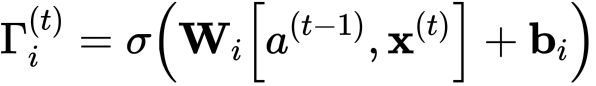
公式的解释:
-
类似于遗忘门(此处为),用sigmoid函数乘后值就落在了0到1之间。
-
将更新门与候选元素逐元素相乘,并将此乘积()用于确定单元状态。
在代码中的变量名:
在代码中,我们将使用学术文献中的变量名。这些变量不使用“ u”表示“更新”。
-
wi是更新门的权重
-
bi是更新门的偏差
-
it是更新门
单元状态
概念:
-
单元状态是传递到未来时间步长的“记忆/内存(memory)”。
-
新单元状态是先前单元状态和候选值的组合。
公式:

公式的解释:
-
之前的单元状态通过遗忘门调整(加权)。
-
候选值通过更新门调整(加权)。
在代码中的变量名:
-
c: 单元状态,包含所有的时间步长,c的shape是(na, m, T)
-
c_next: 下一个时间步长的单元状态,的shape (na, m)
-
c_prev: 之前的单元状态,的shape (na, m)
输出门
概念:
-
输出门决定时间步长要输出的预测值。
-
输出门与其他门一样,它包含从0到1的值。
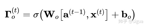
公式:
公式的解释:
-
输出门由之前的隐藏状态和当前的输入 决定。
-
sigmoid函数让值的范围在0到1之间。
在代码中的变量名:
-
wo: 输出门的权重
-
bo: 输出门的偏差
-
ot: 输出门
隐藏状态
概念:
-
隐藏状态将传递到LSTM单元的下一个时间步长。
-
它用于确定下一个时间步长的三个门()。
-
隐藏状态也用于预测。
公式:

公式的解释:
-
隐藏状态由单元状态结合输出门确定。
-
单元状态通过“ tanh”函数把值缩放到-1和+1之间。
-
输出门的作用就像一个“掩码mask”,它既可以保留的值,也可以使这些值不包含在隐藏状态中。
在代码中的变量名:
-
a: 隐藏状态,包含时间步长,shape (na, m, Tx)
-
a_prev: 前一步的隐藏状态,的shape (na, m)
-
a_next: 下一步的隐藏状态,的shape (na, m)
预测值
概念:
-
此用例的预测是分类,所以我们用softmax。
公式:

在代码中的变量名:
-
y_pred: 预测,包含所有的时间步长,的shape (ny, m, Tx),注意,本例中Tx=Ty。
-
yt_pred: 当前时间步长t的预测值,shape是(ny, m)
LSTM cell
一共三个步骤:
1. 连接隐藏状态和输入成一个单独的矩阵
2. 依次计算上面那6个公式
3. 计算预测值
def lstm_cell_forward(xt, a_prev, c_prev, parameters):
"""
Implement a single forward step of the LSTM-cell as described in Figure (4)
Arguments:
xt -- your input data at timestep "t", numpy array of shape (n_x, m).
a_prev -- Hidden state at timestep "t-1", numpy array of shape (n_a, m)
c_prev -- Memory state at timestep "t-1", numpy array of shape (n_a, m)
parameters -- python dictionary containing:
Wf -- Weight matrix of the forget gate, numpy array of shape (n_a, n_a + n_x)
bf -- Bias of the forget gate, numpy array of shape (n_a, 1)
Wi -- Weight matrix of the update gate, numpy array of shape (n_a, n_a + n_x)
bi -- Bias of the update gate, numpy array of shape (n_a, 1)
Wc -- Weight matrix of the first "tanh", numpy array of shape (n_a, n_a + n_x)
bc -- Bias of the first "tanh", numpy array of shape (n_a, 1)
Wo -- Weight matrix of the output gate, numpy array of shape (n_a, n_a + n_x)
bo -- Bias of the output gate, numpy array of shape (n_a, 1)
Wy -- Weight matrix relating the hidden-state to the output, numpy array of shape (n_y, n_a)
by -- Bias relating the hidden-state to the output, numpy array of shape (n_y, 1)
Returns:
a_next -- next hidden state, of shape (n_a, m)
c_next -- next memory state, of shape (n_a, m)
yt_pred -- prediction at timestep "t", numpy array of shape (n_y, m)
cache -- tuple of values needed for the backward pass, contains (a_next, c_next, a_prev, c_prev, xt, parameters)
Note: ft/it/ot stand for the forget/update/output gates, cct stands for the candidate value (c tilde),
c stands for the cell state (memory)
"""
# 从 "parameters" 中取出参数。
Wf = parameters["Wf"] # 遗忘门权重
bf = parameters["bf"]
Wi = parameters["Wi"] # 更新门权重 (注意变量名下标是i不是u哦)
bi = parameters["bi"] # (notice the variable name)
Wc = parameters["Wc"] # 候选值权重
bc = parameters["bc"]
Wo = parameters["Wo"] # 输出门权重
bo = parameters["bo"]
Wy = parameters["Wy"] # 预测值权重
by = parameters["by"]
# 连接 a_prev 和 xt
concat = np.concatenate((a_prev, xt), axis=0)
# 等价于下面代码
# 从 xt 和 Wy 中取出维度
# n_x, m = xt.shape
# n_y, n_a = Wy.shape
# concat = np.zeros((n_a + n_x, m))
# concat[: n_a, :] = a_prev
# concat[n_a :, :] = xt
# 计算 ft (遗忘门), it (更新门)的值
# cct (候选值), c_next (单元状态),
# ot (输出门), a_next (隐藏单元)
ft = sigmoid(np.dot(Wf, concat) + bf) # 遗忘门
it = sigmoid(np.dot(Wi, concat) + bi) # 更新门
cct = np.tanh(np.dot(Wc, concat) + bc) # 候选值
c_next = ft * c_prev + it * cct # 单元状态
ot = sigmoid(np.dot(Wo, concat) + bo) # 输出门
a_next = ot * np.tanh(c_next) # 隐藏状态
# 计算LSTM的预测值
yt_pred = softmax(np.dot(Wy, a_next) + by)
# 用于反向传播的缓存
cache = (a_next, c_next, a_prev, c_prev, ft, it, cct, ot, xt, parameters)
return a_next, c_next, yt_pred, cache
LSTM向前传播
我们已经实现了一个时间步长的LSTM,现在我们可以用for循环对它进行迭代,处理一系列的Tx输入。
LSTM的多个时间步长
指导:
-
从变量x 和 parameters中获得 的维度。
-
初始化三维张量 , 和 .
-
: 隐藏状态, shape
-
: 单元状态, shape
-
: 预测, shape (注意在这个例子里 ).
-
注意 将一个变量设置来和另一个变量相等是"按引用复制". 换句话说,就是不用使用c = a, 否则这两个变量指的是同一个变量,更改任何其中一个变量另一个变量的值都会跟着变。
-
初始化二维张量
-
储存了t时间步长的隐藏状态,它的变量名是a_next。
-
, 时间步长0时候的初始隐藏状态,调用该函数时候传入的值,它的变量名是a0。
-
和 代表单个时间步长,所以他们的shape都是
-
通过传入函数的初始化隐藏状态来初始化 。
-
用0来初始化 。
-
变量名是 c_next.
-
表示单个时间步长, 所以它的shape是
-
注意: create c_next as its own variable with its own location in memory. 不要将它通过3维张量的切片来初始化,换句话说, 不要 c_next = c[:,:,0].
-
对每个时间步长,做以下事情:
-
从3维的张量 中, 获取在时间步长t处的2维切片 。
-
调用你之前定义的 lstm_cell_forward 函数,获得隐藏状态,单元状态,预测值。
-
存储隐藏状态,单元状态,预测值到3维张量中。
-
把缓存加入到缓存列表。
def lstm_forward(x, a0, parameters):
"""
Implement the forward propagation of the recurrent neural network using an LSTM-cell described in Figure (4).
Arguments:
x -- Input data for every time-step, of shape (n_x, m, T_x).
a0 -- Initial hidden state, of shape (n_a, m)
parameters -- python dictionary containing:
Wf -- Weight matrix of the forget gate, numpy array of shape (n_a, n_a + n_x)
bf -- Bias of the forget gate, numpy array of shape (n_a, 1)
Wi -- Weight matrix of the update gate, numpy array of shape (n_a, n_a + n_x)
bi -- Bias of the update gate, numpy array of shape (n_a, 1)
Wc -- Weight matrix of the first "tanh", numpy array of shape (n_a, n_a + n_x)
bc -- Bias of the first "tanh", numpy array of shape (n_a, 1)
Wo -- Weight matrix of the output gate, numpy array of shape (n_a, n_a + n_x)
bo -- Bias of the output gate, numpy array of shape (n_a, 1)
Wy -- Weight matrix relating the hidden-state to the output, numpy array of shape (n_y, n_a)
by -- Bias relating the hidden-state to the output, numpy array of shape (n_y, 1)
Returns:
a -- Hidden states for every time-step, numpy array of shape (n_a, m, T_x)
y -- Predictions for every time-step, numpy array of shape (n_y, m, T_x)
c -- The value of the cell state, numpy array of shape (n_a, m, T_x)
caches -- tuple of values needed for the backward pass, contains (list of all the caches, x)
"""
# 初始化 "caches", 用来存储每个时间步长的cache值的
caches = []
Wy = parameters['Wy']
# 从 x 和 parameters['Wy'] 的shape中获取纬度值
n_x, m, T_x = x.shape
n_y, n_a = Wy.shape
# 初始化 "a", "c" and "y"
a = np.zeros((n_a, m, T_x))
c = np.zeros((n_a, m, T_x))
y = np.zeros((n_y, m, T_x))
# 初始化 a_next and c_next
a_next = a0
c_next = np.zeros(a_next.shape)
# loop over all time-steps
for t in range(T_x):
# 从3维张量x中获取t时间步长的2维张量xt
xt = x[:, :, t]
# 更新下一个时间步长的隐藏状态, 下一个单元状态, 计算预测值
a_next, c_next, yt, cache = lstm_cell_forward(xt, a_next, c_next, parameters)
# 把下一个时间步长长的隐藏状态保存起来
a[:,:,t] = a_next
# 把下一个时间步长长的单元状态保存起来
c[:,:,t] = c_next
# 把预测值保存起来
y[:,:,t] = yt
# 保存缓存值
caches.append(cache)
# 用于向后传播
caches = (caches, x)
return a, y, c, caches
恭喜你!现在,你已经为LSTM实现了前向传播。使用深度学习框架时,实施前向传播足以构建出色性能的系统。