下面文章描述可能比excel高级一点,距离backtrader这些框架又差一点。做最基础的测试可以,如果后期加入加仓功能,或者是止盈止损等功能,很不合适。只能做最简单的技术指标测试。
导包,常用包导入:
import os
import akshare as ak
import requests
import numpy as np
import pandas as pd
import matplotlib.pyplot as plt
import talib as ta
%matplotlib inline
plt.style.use("ggplot")
获取数据,本文使用akshare中债券数据为对象分析:
bond_zh_hs_daily_df = ak.bond_zh_hs_daily(symbol="sh010107")
添加指标:
def backtest_trend_strategy(ohlc: pd.DataFrame,
                            fast_period: int = 50,
                            slow_period: int = 200,
                            threshold: float = 1.0) -> pd.DataFrame:
    """封装向量化回测的逻辑"""
    # 计算指标
    ohlc["fast_ema"] = talib.EMA(ohlc.close, fast_period)
    ohlc["slow_ema"] = talib.EMA(ohlc.close, slow_period)
    ohlc["pct_diff"] = (ohlc["fast_ema"] / ohlc["slow_ema"] - 1) * 100

    # 生成信号,1表示做多,-1表示做空,0表示空仓
    ohlc["signal"] = np.where(ohlc["pct_diff"] > threshold, 1, 0)
    ohlc["signal"] = np.where(ohlc["pct_diff"] < -threshold, -1, ohlc["signal"])

    # 计算策略收益率
    ohlc["returns"] = np.log(ohlc["close"] / ohlc["close"].shift(1))
    ohlc["strategy"] = ohlc["signal"].shift(1) * ohlc["returns"]
    ohlc["strategy_returns"] = ohlc["strategy"].cumsum()

    return ohlc
运行策略,并绘制图片:
data = strategy1(data)


fig, ax = plt.subplots(nrows=3, ncols=1, figsize=(12, 15), sharex=True)

ax[0].plot(data.index, data["close"])
ax[0].plot(data.index, data["fast_ema"])
ax[0].plot(data.index, data["slow_ema"])
ax[0].set_title("Price and Indicators")

ax[1].plot(data.index, data["signal"])
ax[1].set_title("Strategy Position")

data[["returns", "strategy"]].cumsum().plot(ax=ax[2], title="Strategy Return")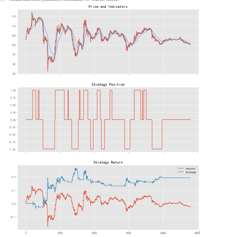
参数优化:
# 选择核心参数和扫描区间,其它参数保持不变
fast_period_rng = np.arange(5, 101, 5)

total_return = []
for fast_period in fast_period_rng:
    ohlc = data.filter(["open", "high", "low", "close"])
    res = backtest_trend_strategy(ohlc, fast_period, 200, 1.0)
    total_return.append(res["strategy_returns"].iloc[-1])


# 散点图:策略收益率 vs 快速均线回溯期
fig, ax = plt.subplots(figsize=(12, 7))
ax.plot(fast_period_rng, total_return, "r-o", markersize=10)
ax.set_title("Strategy Return vs Fast period")
ax.set_xlabel("fast_period")
ax.set_ylabel("return(%)")