联邦学习(Federated Learning) 是人工智能的一个新的分支,这项技术是谷歌2016年于论文
Communication-Efficient Learning of Deep Networks from Decentralized Data中首次提出。
在我的另一篇博文联邦学习:《Communication-Efficient Learning of Deep Networks from Decentralized Data中详细解析了该篇论文,而本篇博文的目的是利用这篇解读文章对原始论文中的FedAvg方法进行复现。
因此,阅读本文前建议先阅读联邦学习:《Communication-Efficient Learning of Deep Networks from Decentralized Data。
联邦学习中存在多个客户端,每个客户端都有自己的数据集,这个数据集他们是不愿意共享的。
本文选用的数据集为中国北方某城市十个区/县从2016年到2019年三年的真实用电负荷数据,采集时间间隔为1小时,即每一天都有24个负荷值。
我们假设这10个地区的电力部门不愿意共享自己的数据,但是他们又想得到一个由所有数据统一训练得到的全局模型。
除了电力负荷数据意外,还有风功率数据,两个数据通过参数type指定:type == 'load’表示负荷数据,'wind’表示风功率数据。
用某一时刻前24个时刻的负荷值以及该时刻的相关气象数据(如温度、湿度、压强等)来预测该时刻的负荷值。
对于风功率数据,同样使用某一时刻前24个时刻的风功率值以及该时刻的相关气象数据来预测该时刻的风功率值。
各个地区应该就如何制定特征集达成一致意见,本文使用的各个地区上的数据的特征是一致的,可以直接使用。
原始论文中提出的FedAvg的框架为:
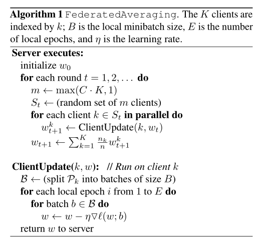
由于本文中需要利用各个客户端的模型参数来对服务器端的模型参数进行更新,因此本文决定采用numpy搭建一个四层的神经网络模型。模型的具体搭建过程可以参考上一篇博文:从矩阵链式求导的角度来深入理解BP算法(原理+代码)。在这篇博文里面我详细得介绍了神经网络参数更新的过程,这将有助于理解本文中的模型参数更新过程。
神经网络由1个输入层、3个隐藏层以及1个输出层组成,激活函数全部采用Sigmoid函数。
网络各层间的运算关系,也就是前向传播过程如下所示:

因此,客户端参数更新实际上就是更新四个 w。
服务器端执行以下步骤:

简单来说,每一轮通信时都只是选择部分客户端,这些客户端利用本地的数据进行参数更新,然后将更新后的参数传给服务器,服务器汇总客户端更新后的参数形成最新的全局参数。下一轮通信时,服务器端将最新的参数分发给被选中的客户端,进行下一轮更新。
客户端没什么可说的,就是利用本地数据对神经网络模型的参数进行更新。
参数:
代码实现:
class FedAvg:
    def __init__(self, options):
        self.C = options['C']
        self.E = options['E']
        self.B = options['B']
        self.K = options['K']
        self.r = options['r']
        self.clients = options['clients']
        self.type = options['type']
        self.lr = options['lr']
        self.input_dim = options['input_dim']
        self.nn = BP(file_name='server', B=B, E=E, input_dim=self.input_dim, type=self.type, lr=self.lr)
        self.nns = []
        # distribution
        for i in range(self.K):
            s = copy.deepcopy(self.nn)
            s.file_name = self.clients[i]
            self.nns.append(s)
其中 self.nn是服务器端初始化的全局参数,由于服务器端不需要进行反向传播更新参数,因此不需要定义各个隐层以及输出。
服务器端代码如下:
def server(self):
     for t in range(self.r):
          print('第', t + 1, '轮通信:')
          m = np.max([int(self.C * self.K), 1])
          # sampling
          index = random.sample(range(0, self.K), m)
          # dispatch
          self.dispatch(index)
          # local updating
          self.client_update(index)
          # aggregation
          self.aggregation(index)

     # return global model
     return self.nn
其中client_update(index):
def client_update(self, index):  # update nn
     for k in index:
          self.nns[k] = train(self.nns[k])
aggregation(index):
def aggregation(self, index):
     # update w
     s = 0
     for j in index:
          # normal
          s += self.nns[j].len

     w1 = np.zeros_like(self.nn.w1)
     w2 = np.zeros_like(self.nn.w2)
     w3 = np.zeros_like(self.nn.w3)
     w4 = np.zeros_like(self.nn.w4)

     for j in index:
          # normal
          w1 += self.nns[j].w1 * (self.nns[j].len / s)
          w2 += self.nns[j].w2 * (self.nns[j].len / s)
          w3 += self.nns[j].w3 * (self.nns[j].len / s)
          w4 += self.nns[j].w4 * (self.nns[j].len / s)
     # update server
     self.nn.w1, self.nn.w2, self.nn.w3, self.nn.w4 = w1, w2, w3, w4
dispatch(index):
def aggregation(self, index):
     # update w
     s = 0
     for j in index:
          # normal
          s += self.nns[j].len

     w1 = np.zeros_like(self.nn.w1)
     w2 = np.zeros_like(self.nn.w2)
     w3 = np.zeros_like(self.nn.w3)
     w4 = np.zeros_like(self.nn.w4)

     for j in index:
          # normal
          w1 += self.nns[j].w1 * (self.nns[j].len / s)
          w2 += self.nns[j].w2 * (self.nns[j].len / s)
          w3 += self.nns[j].w3 * (self.nns[j].len / s)
          w4 += self.nns[j].w4 * (self.nns[j].len / s)
     # update server
     self.nn.w1, self.nn.w2, self.nn.w3, self.nn.w4 = w1, w2, w3, w4
下面对重要代码进行分析:
客户端的选择
m = np.max([int(self.C * self.K), 1])
index = random.sample(range(0, self.K), m)
index中存储中m个0~10间的整数,表示被选中客户端的序号。
客户端的更新
for k in index:
    self.client_update(self.nns[k])
服务器端汇总客户端模型的参数
关于模型汇总方式,可以参考一下我的另一篇文章:对FedAvg中模型聚合过程的理解。
当然,这只是一种很简单的汇总方式,还有一些其他类型的汇总方式。论文Electricity Consumer Characteristics Identification: A Federated Learning Approach中总结了三种汇总方式:
将更新后的参数分发给客户端
def dispatch(self, inidex):
     # dispatch
     for i in index:
          self.nns[i].w1, self.nns[i].w2, self.nns[i].w3, self.nns[
               i].w4 = self.nn.w1, self.nn.w2, self.nn.w3, self.nn.w4
客户端只需要利用本地数据来进行更新就行了:
def client_update(self, index):  # update nn
     for k in index:
          self.nns[k] = train(self.nns[k])
其中train():
def train(nn):
    print('training...')
    if nn.type == 'load':
        train_x, train_y, test_x, test_y = nn_seq(nn.file_name, nn.B, nn.type)
    else:
        train_x, train_y, test_x, test_y = nn_seq_wind(nn.file_name, nn.B, nn.type)
    nn.len = len(train_x)
    batch_size = nn.B
    epochs = nn.E
    batch = int(len(train_x) / batch_size)
    for epoch in range(epochs):
        for i in range(batch):
            start = i * batch_size
            end = start + batch_size
            nn.forward_prop(train_x[start:end], train_y[start:end])
            nn.backward_prop(train_y[start:end])
        print('当前epoch:', epoch, ' error:', np.mean(nn.loss))
    return nn
def global_test(self):
     model = self.nn
     c = clients if self.type == 'load' else clients_wind
     for client in c:
          model.file_name = client
          test(model)
本次实验的参数选择为:
| K | C | E | B | r |
|---|---|---|---|---|
| 10 | 0.5 | 50 | 50 | 5 |
if __name__ == '__main__': K, C, E, B, r = 10, 0.5, 50, 50, 5 type = 'load' input_dim = 30 if type == 'load' else 28 _client = clients if type == 'load' else clients_wind lr = 0.08 options = {<!--{C}%3C!%2D%2D%20%2D%2D%3E-->'K': K, 'C': C, 'E': E, 'B': B, 'r': r, 'type': type, 'clients': _client, 'input_dim': input_dim, 'lr': lr} fedavg = FedAvg(options) fedavg.server() fedavg.global_test()if __name__ == '__main__':
    K, C, E, B, r = 10, 0.5, 50, 50, 5
    type = 'load'
    input_dim = 30 if type == 'load' else 28
    _client = clients if type == 'load' else clients_wind
    lr = 0.08
    options = {'K': K, 'C': C, 'E': E, 'B': B, 'r': r, 'type': type, 'clients': _client,
               'input_dim': input_dim, 'lr': lr}
    fedavg = FedAvg(options)
    fedavg.server()
    fedavg.global_test()
各个客户端单独训练(训练50轮,batch大小为50)后在本地的测试集上的表现为:
| 客户端编号 | 1 | 2 | 3 | 4 | 5 | 6 | 7 | 8 | 9 | 10 |
|---|---|---|---|---|---|---|---|---|---|---|
| MAPE / % | 5.79 | 6.73 | 6.18 | 5.82 | 5.49 | 4.55 | 6.23 | 9.59 | 4.84 | 5.49 |
可以看到,由于各个客户端的数据都十分充足,所以每个客户端自己训练的本地模型的预测精度已经很高了。
服务器与客户端通信5轮后,服务器上的全局模型在10个客户端测试集上的表现如下所示:
| 客户端编号 | 1 | 2 | 3 | 4 | 5 | 6 | 7 | 8 | 9 | 10 |
|---|---|---|---|---|---|---|---|---|---|---|
| MAPE / % | 6.58 | 4.19 | 3.17 | 5.13 | 3.58 | 4.69 | 4.71 | 3.75 | 2.94 | 4.77 |
可以看到,经过联邦学习框架得到全局模型在各个客户端上表现同样很好,这是因为十个地区上的数据是独立同分布的。
我把数据和代码放在了GitHub上:FedAvg