自然语言处理的核心概念之一是如何量化单词和表达式,以便能够在模型环境中使用它们。语言元素到数值表示的这种映射称为词嵌入。
Word2Vec是一个词嵌入过程。这个概念相对简单:通过一个句子一个句子地在语料库中循环去拟合一个模型,根据预先定义的窗口中的相邻单词预测当前单词。
为此,它使用了一个神经网络,但实际上最后我们并不使用预测的结果。一旦模型被保存,我们只保存隐藏层的权重。在我们将要使用的原始模型中,有300个权重,因此每个单词都由一个300维向量表示。
请注意,两个单词不必彼此接近的地方才被认为是相似的。如果两个词从来没有出现在同一个句子中,但它们通常被相同的包围,那么可以肯定它们有相似的意思。
Word2Vec中有两种建模方法:skip-gram和continuous bag of words,这两种方法都有各自的优点和对某些超参数的敏感性。
当然,你得到的词向量取决于你训练模型的语料库。一般来说,你确实需要一个庞大的语料库,有维基百科上训练过的版本,或者来自不同来源的新闻文章。我们将要使用的结果是在Google新闻上训练出来的。
自定义一个很小的语料库,尝试给出Word2Vec的简单可视化:
import gensim

%matplotlib inline
from gensim.models import Word2Vec
from sklearn.decomposition import PCA
from matplotlib import pyplot

# 训练的语料
sentences = [['this', 'is', 'the', 'an', 'apple', 'for', 'you'],
             ['this', 'is', 'the', 'an', 'orange', 'for', 'you'],
             ['this', 'is', 'the', 'an', 'banana', 'for', 'you'],
             ['apple','is','delicious'],
             ['apple','is','sad'],
             ['orange','is','delicious'],
             ['orange','is','sad'],
             ['apple','tests','delicious'],
             ['orange','tests','delicious']]

# 利用语料训练模型
model = Word2Vec(sentences,window=5, min_count=1)

# 基于2d PCA拟合数据
# X = model[model.wv.vocab]
X = model.wv[model.wv.key_to_index]
pca = PCA(n_components=2)
result = pca.fit_transform(X)

# 可视化展示
pyplot.scatter(result[:, 0], result[:, 1])
words = list(model.wv.key_to_index)
for i, word in enumerate(words):
    pyplot.annotate(word, xy=(result[i, 0], result[i, 1]))
pyplot.show()
因为语料库是随机给出的,并且数量很少,所以训练出来的词向量展示出来的词和词之间的相关性不那么强。这里主要是想表明假如我们输入一系列单词,通过Word2Vec模型可以得到什么样的输出。
通过已经在Google新闻的语料上训练好的模型来看看Word2Vec得到的词向量都可以怎么使用。
首先需要下载预训练Word2Vec向量,这可以从各种各样的背景领域中进行选择。基于Google新闻语料库的训练模型可通过搜索“Google News vectors negative 300”来下载。这个文件大小是1.53GB,包含了30亿单词的300维表示。
和上述在Python中的简单可视化一样,需要使用gensim库。假设刚才下载好的文件保存在电脑的E盘的“wordpretrain”文件夹中。
from gensim.models.keyedvectors import KeyedVectors

word_vectors = KeyedVectors.load_word2vec_format(\
    'E:\wordpretrain/GoogleNews-vectors-negative300.bin.gz', \
    binary = True, limit = 1000000)
如此,便拥有了一个现成的词向量模型,亦即每个单词都由一个300维的向量唯一表示。下面我们来看看关于它的一些简单用法。
1、可以实际查看任意单词的向量表示:
word_vectors['dog']
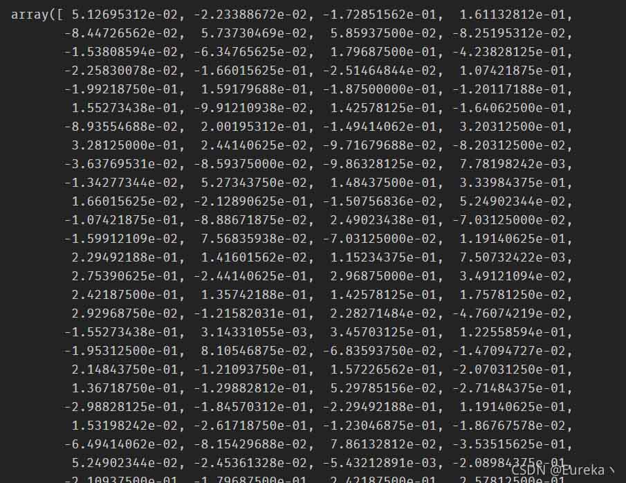
但很难解释这个向量的每一维代表什么意思。
2、可以使用most_similar函数找到意思相近的单词,topn参数定义要列出的单词数:
word_vectors.most_similar(positive = ['nice'], topn = 5)
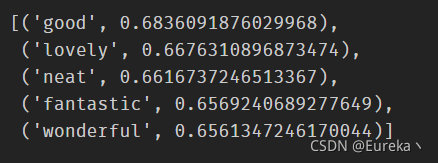
括号中的数字表示相似度的大小。
3、如果我们想合并father和woman这两个单词的向量,并减去man这个单词的向量,可以得到:
word_vectors.most_similar(
positive = ['father', 'woman'], negative = ['man'], topn = 1)
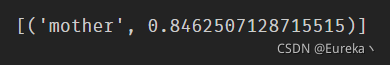
其实这件事情很容易想到:假设在两个维度(亲子关系和性别)下,“woman”这个单词的向量为(0,1),“man”的向量为(0,-1),“father”的向量为(1,-1),“mother”的向量为(1,1),那么“father”+“woman”-“man”= (1,-1) + (0,1) - (0,-1) = (1,1) =“mother”。当然,区别在于这里我们有300个维度,但原理上是相同的。
4、可视化:
%matplotlib inline
import pandas as pd
import matplotlib.pyplot as plt
import seaborn as sns
from sklearn.decomposition import PCA
import adjustText
from jupyterthemes import jtplot
jtplot.style(theme='onedork') #选择一个绘图主题
def plot_2d_representation_of_words(
    word_list,
    word_vectors,
    flip_x_axis = False,
    flip_y_axis = False,
    label_x_axis = "x",
    label_y_axis = "y",
    label_label = "fruit"):

    pca = PCA(n_components = 2)

    word_plus_coordinates=[]

    for word in word_list:
        current_row = []
        current_row.append(word)
        current_row.extend(word_vectors[word])
        word_plus_coordinates.append(current_row)

    word_plus_coordinates = pd.DataFrame(word_plus_coordinates)

    coordinates_2d = pca.fit_transform(
        word_plus_coordinates.iloc[:,1:300])
    coordinates_2d = pd.DataFrame(
        coordinates_2d, columns=[label_x_axis, label_y_axis])
    coordinates_2d[label_label] = word_plus_coordinates.iloc[:,0]
    if flip_x_axis:
        coordinates_2d[label_x_axis] = \
        coordinates_2d[label_x_axis] * (-1)
    if flip_y_axis:
        coordinates_2d[label_y_axis] = \
        coordinates_2d[label_y_axis] * (-1)

    plt.figure(figsize = (15,10))
    p1=sns.scatterplot(
        data=coordinates_2d, x=label_x_axis, y=label_y_axis)

    x = coordinates_2d[label_x_axis]
    y = coordinates_2d[label_y_axis]
    label = coordinates_2d[label_label]

    texts = [plt.text(x[i], y[i], label[i]) for i in range(len(x))]
    adjustText.adjust_text(texts)
fruits = ['apple','orange','banana','lemon','car','tram','boat','bicycle',
'cherry','mango','grape','durian','watermelon','train','motorbike','ship',
'peach','pear','pomegranate','strawberry','bike','bus','truck','subway','airplane']plot_2d_representation_of_words(
word_list = fruits,
word_vectors = word_vectors,
flip_y_axis = True)
这里我在水果类的单词列表中混入了少许交通工具类的单词。显然,结果还算不错,不仅能明显看到单词之间的相关性,还能自动聚类。
当然,上述只是Word2Vec模型的简单操作和应用,其既可以执行词语层面的任务,也可以作为很多模型的输入,包括但不限于:
· 计算相似度
· 作为SVM/LSTM等模型的输入
· 句子表示
· 文档表示
从上述Word2Vec实操和简单应用来看,我们可以得出其词向量训练的核心思想:若两个单词出现的语境相似,则它们的向量也相似。
以上为个人经验,希望能给大家一个参考,也希望大家多多支持。