ais解码

The AI community has a serious problem: 87% of our projects never make it to production. If another field had that kind of failure rate, we might not call it science at all. What exactly are we missing?

AI社区存在一个严重的问题：我们87％的项目从未投入生产。如果另一个领域的失败率如此之高，我们可能根本就不称之为科学。我们到底缺少什么？

· We are not short on data: We generate 1.7 MB per person per second in 2020

·我们并不缺乏数据：到2020年，我们每人每秒产生1.7 MB

· We are not short on theoretical advances: 31 new AI papers were published on Arxiv just today

·我们在理论上不乏不足：仅在今天的Arxiv上发表了31篇新的AI论文

· We are not short on investment: It’s expected to top £150 billion by 2025

·我们并不缺乏投资：到2025年，预计将突破1500亿英镑

· We are not short on performance: AI compute performance has been doubling every 3.4 months

·我们的性能并不缺：AI计算性能每3.4个月翻一番

What we are short on is trust. Modern AI/ML techniques such as deep learning and tree-based methods can deliver great accuracy but are also harder to interpret than older regression-based methods. Our model might tell the future with perfect accuracy, but if the experts we serve see it as a black box, it will not make it beyond the lab. If end users don’t trust our model, they will ignore it, just as the ancient Greeks ignored Cassandra’s accurate prophesies.

我们缺乏的是信任 。诸如深度学习和基于树的方法之类的现代AI / ML技术可以提供较高的准确性，但也比旧的基于回归的方法更难解释。我们的模型可能会以完美的准确性告诉未来，但是如果我们所服务的专家将其视为黑匣子，那么它将无法超出实验室的范围。如果最终用户不信任我们的模型，他们将忽略它，就像古希腊人忽略了卡桑德拉的准确预言一样。

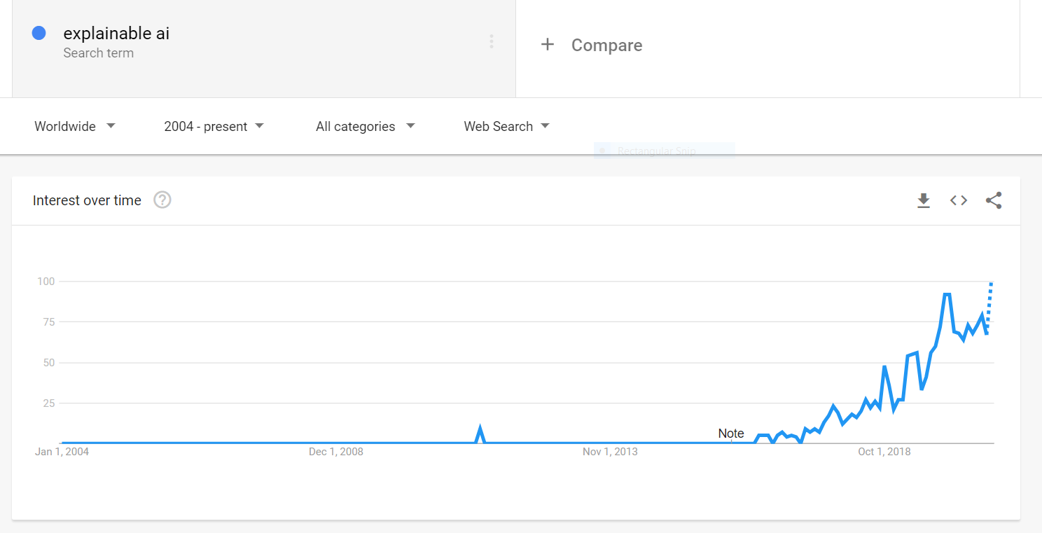
Explainable AI (XAI) is a set of technologies that seek to make complex models understandable and trustworthy. Interest has been growing rapidly over the past two years:

可解释的AI (XAI)是一组旨在使复杂的模型易于理解和值得信赖的技术。在过去两年中，兴趣Swift增长：

Image for post — Source: Google Trends. Image by Author

You can find lots of articles introducing XAI. I’ve included some of my favorites in the footnotes below. However, they mostly focus on the how at the expense of the why, and are light on realistic data and domain expertise.

您可以找到很多介绍XAI的文章。我在下面的脚注中包含了一些我的最爱。但是，他们主要集中在how 上，而why却为此付出了代价，并且对实际数据和领域专业知识有所了解。

This article will illustrate how XAI fits into the AI/ML workflow with a case study: A credit model I developed as part of the Kaggle Home Credit competition. The training dataset consists of 397,511 loan applications from prospective borrowers. The model seeks to predict which borrowers will default. It was built with LightGBM, a tree-based algorithm.

本文将通过案例研究说明XAI如何适合AI / ML工作流程：我在Kaggle Home Credit竞赛中开发的一种信用模型。培训数据集包括来自潜在借款人的397,511笔贷款申请。该模型试图预测哪些借款人将违约。它是使用LightGBM(一种基于树的算法)构建的。

In our consulting practice at Genpact, we see three major XAI uses cases. Let’s go through each one.

在Genpact的咨询实践中，我们看到了三个主要的XAI用例。让我们逐一进行。

1.开发人员：提高模型性能 (1. Developer: Improve Model Performance)

A model developer would like to use XAI to

模型开发人员想使用XAI来

· Eliminate features that do not add much value, making the model lighter, faster to train and less likely to overfit

·消除不会增加太多价值的功能，从而使模型更轻巧，训练更快且不太可能过拟合

· Ensure the model is relying on features that make sense from a domain perspective. For example, we don’t want the model to use the borrower’s first name to predict loan defaults

·确保模型依赖于从领域角度来看有意义的功能。例如，我们不希望模型使用借款人的名字来预测贷款违约

Most tree-based libraries include a basic feature importance report that can help with these tasks. Here it is for our credit model:

大多数基于树的库都包含基本功能重要性报告，可以帮助完成这些任务。这是我们的信用模型：

How should we read this chart?

我们应该如何阅读此图表？

· The most important features are on top

·最重要的功能在最前面

· Feature importance is defined by how frequently it is used by the model’s trees (by split) or by how much signal it adds (by gain)

·功能重要性的定义是通过模型树的使用频率(通过拆分)或信号添加的信号数量(通过增益)来定义

What is it telling us?

它告诉我们什么？

· The most important feature is NEW_EXT_SOURCES_MEAN. This represents the borrower’s credit score, similar to a FICO score in the US. Technically, it is the average of three scores from external credit bureaus

·最重要的功能是NEW_EXT_SOURCES_MEAN。这代表借款人的信用评分，类似于美国的FICO评分。从技术上讲，它是来自外部征信机构的三个分数的平均值

· The average credit score is more important than any of the individual scores (EXT_SOURCE_1, 2, 3)

·平均信用评分比任何单个评分都重要(EXT_SOURCE_1，2，3)

· The second most important feature is the applicant’s age, DAYS_BIRTH, etc.

·第二个最重要的功能是申请人的年龄，DAYS_BIRTH等。

So what?

所以呢？

· We can use this to improve model performance. For example, we see all three credit scores are important (EXT_SOURCE 1, 2, and 3) but the mean is the most important. Therefore, there is some difference between scores that the model is trying to learn. We can make that explicit by engineering features for that difference, e.g. EXT_SOURCE_1 — EXT_SOURCE_2.

·我们可以使用它来改善模型性能。例如，我们看到所有三个信用评分都很重要(EXT_SOURCE 1、2和3)，但均值是最重要的。因此，模型试图学习的分数之间存在一些差异。我们可以通过工程特性来明确表示该差异，例如EXT_SOURCE_1 — EXT_SOURCE_2。

· We can use this to validate model logic, to a limited degree. For example, are we comfortable relying on the borrower age this much? This is hard to answer because we still don’t know just how the model is using borrower age.

·我们可以在一定程度上使用它来验证模型逻辑。例如，我们是否足够放心地依赖借款人年龄？这很难回答，因为我们仍然不知道该模型如何使用借款人年龄。

Compare this against a similar report generated by an XAI package called SHAP:

将此与XAI软件包SHAP生成的类似报告进行比较：

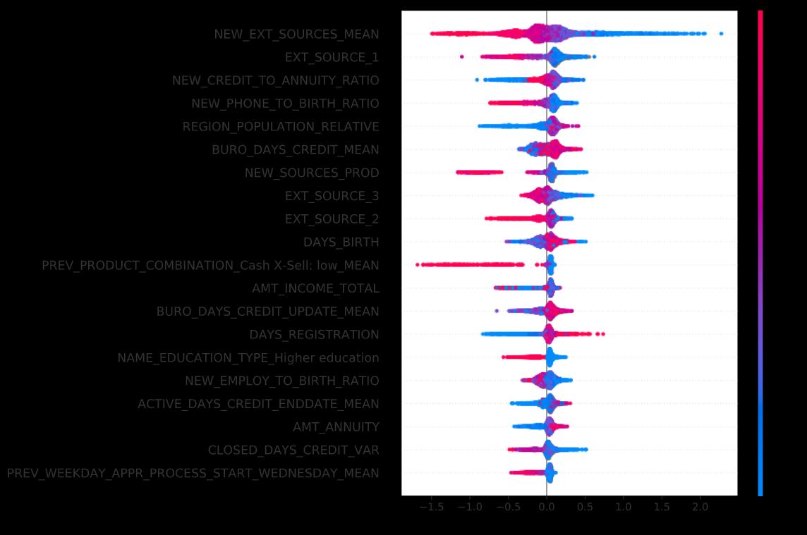
Both charts show the model’s most “important” features on top, though they don’t quite agree on the order. Many believe the SHAP order is more accurate. In any event, the SHAP chart provides a lot more detail.

这两个图表在顶部都显示了模型最“重要”的功能，尽管它们在顺序上不太一致。许多人认为SHAP顺序更准确。无论如何，SHAP图表会提供更多详细信息。

How should we read this chart?

我们应该如何阅读此图表？

Let’s zoom in on the top feature:

让我们放大最重要的功能：

· Top-Down Position: This is the feature that “moves the needle” the most for the model’s output. It is the most impactful.

· 自上而下的位置：此功能可以最大程度地“移动针”，以达到模型输出的目的。这是最有影响力的。

· Color: To the right of the feature label, we see a violin-shaped dot plot. Each dot represents a borrower in our dataset. Blue dots represent borrowers with low credit scores (risky). Red dots are high credit scores (safe). The same blue-red scale applies to all quantitative features.

· 颜色：在功能标签的右侧，我们看到一个小提琴形的点状图。每个点代表我们数据集中的借款人。蓝点表示信用评分较低(风险)的借款人。红点是高信用评分(安全)。相同的蓝红色标度适用于所有定量特征。

· Left-Right Position: Dots to the left of the center-line represent borrowers whose credit scores decrease the model output, i.e. reduce the predicted probability of default. Dots to the right are those for whom the credit score increases the model output.

· 左右位置：中心线左侧的点表示借款人，其信用评分会降低模型输出，即降低预测的违约概率。右边的点是那些信用评分增加模型输出的点。

What is it telling us?

它告诉我们什么？

· The dots on the left are mostly red, meaning that high credit scores (red) tend to decrease the probability of default (left).

·左侧的点大多是红色的，这意味着较高的信用评分(红色)会降低违约的可能性(左侧)。

So what?

所以呢？

· We can use this to debug the model. For example, if one of the credit bureaus reported a score where high values are risky and low values safe, or if we had mixed up the probability of default with the probability of repayment, this chart would show the problem and allow us to fix it. This happens more often than one might think.

·我们可以使用它来调试模型。例如，如果其中一个征信机构报告了高风险值和低风险值的分数，或者如果我们将违约概率与还款概率混合在一起，则此图表将显示问题并允许我们解决。这种情况发生的频率比人们想象的要多。

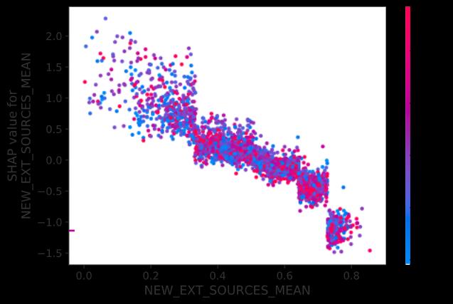
Let’s zoom in further on that last point. Here is a chart that shows how credit scores affect the predicted probability of default.

让我们进一步放大最后一点。这是一张图表，显示信用评分如何影响预测的违约概率。

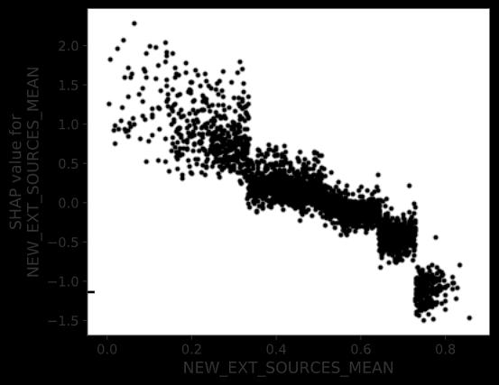
How should we read this chart?

我们应该如何阅读此图表？

· As before, each dot represents a borrower.

·和以前一样，每个点都代表借款人。

· The horizontal axis is the credit score, scaled from zero to one.

·横轴是信用分数，从0缩放到1。

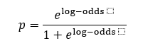
· The vertical axis is not the predicted probability of default, but the contribution of the credit score to that probability. It is scaled as log-odds rather than probability units, same as the raw output from our logistic model. See footnotes for the formula to convert log-odds to probability.

·纵轴不是预测的违约概率，而是信用评分对该概率的贡献。它按对数奇数而不是概率单位进行缩放，与我们的逻辑模型的原始输出相同。有关将对数奇数转换为概率的公式，请参见脚注。

What is it telling us?

它告诉我们什么？

· This scatterplot slopes from top left to the bottom right because low credit scores (left) increase the predicted probability of default (top) and high credit scores (right) decrease it (bottom).

·此散点图从左上方到右下方倾斜，因为低信用评分(左)增加了预测的违约概率(顶部)，而高信用评分(右)则降低了预测的概率(底部)。

So what?

所以呢？

· If our model was linear, the dots would slope down in a perfect line.

·如果我们的模型是线性的，则点将沿一条完美的线向下倾斜。

· We see a thicker scatterplot instead because our model includes feature interactions. The same credit score (vertical line) can affect two borrowers differently, depending on the value of another feature.

·我们看到的是散点图更粗，因为我们的模型包括要素交互。相同的信用评分(垂直线)可能会影响另一个借款人，具体取决于另一个功能的价值。

Let’s add some interaction data to the chart:

让我们向图表添加一些交互数据：

How should we read this chart?

我们应该如何阅读此图表？

· Note that the axes haven’t changed, and the dots haven’t moved.

·请注意，轴未更改，圆点也未移动。

· We have only added a color scale based on a second (interaction) feature, NEW_CREDIT_TO_ANNUITY_RATIO. This is the ratio between the requested loan amount and the annual loan payment. The lower that ratio (blue) the safer the loan is considered because it should take less time to pay off.

·我们仅添加了基于第二个(交互)功能的色标NEW_CREDIT_TO_ANNUITY_RATIO。这是请求的贷款额与年度贷款额之间的比率。该比率(蓝色)越低，则认为贷款越安全，因为还清时间应更少。

What is it telling us?

它告诉我们什么？

· Unfortunately, the color doesn’t tell us much: the blue and red dots seem randomly dispersed. This means there is no clear interaction between the two features we plotted. However, consider the following interaction plot:

·不幸的是，颜色并不能告诉我们太多：蓝色和红色的点似乎是随机分散的。这意味着我们绘制的两个特征之间没有明确的交互作用。但是，请考虑以下交互图：

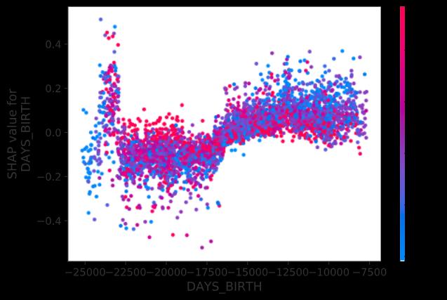
How should we read this chart?

我们应该如何阅读此图表？

· The color scale represents the same feature as before, but now we’ve switched the horizontal axis from credit score to the borrower’s age, expressed as the number of days from today counting back to their birth, hence a negative number.

·色标表示与以前相同的功能，但是现在我们将水平轴从信用评分切换为借款人的年龄，表示为从今天算起到其出生的天数，因此为负数。

· Ages range from 21 years on the right (7,500/365=20.5) to 68 years on the left (25,000/365=68.5).

·年龄范围从右边的21岁(7,500 / 365 = 20.5)到左边的68岁(25,000 / 365 = 68.5)。

· The vertical axis, shows the impact of the borrower’s age on the predicted default probability, expressed as log-odds.

·垂直轴，显示了借款人的年龄对预测违约概率的影响，表现为对数的赔率。

What is this chart telling us?

这张图告诉我们什么？

· The big picture is that older borrowers are generally safer (lower) than younger borrowers. This is true up until you hit age 65 or so (-23,000 days). Past that age, there is a wide dispersion. Senior citizen credit quality is all over the place, but the new credit to annuity ratio plays a big role, the lower the better.

·总体情况是，老年借款人通常比年轻借款人更安全(较低)。直到您达到65岁左右(-23,000天)，情况才如此。超过那个年龄，分布广泛。老年人的信用质量无处不在，但是新的信用年金比率起着很大的作用，越低越好。

· More subtly: Something interesting happens around age 45 (-16,250 days). For borrowers younger than 45 (right), blue dots are generally higher than red dots. In credit terms, younger borrowers asking for short term loans (low credit to annual payment = blue) are riskier. For older borrowers (left), the relationship is reversed, with long term loans becoming riskier.

·更巧妙：45岁左右(-16250天)发生了一些有趣的事情。对于未满45岁(右)的借款人，蓝点通常高于红点。从信贷角度来看，年轻的借款人要求短期贷款(对年付的低信贷=蓝色) 更具风险。 对于年龄较大的借款人(左)，这种关系是相反的，长期贷款的风险更高。

So what?

所以呢？

· I’m not sure why the Home Credit dataset exhibits this pattern. It might be the result of a lending policy, a product characteristic or it could be accidental. If this were a real credit model, I would discuss this pattern with a domain expert (an underwriter in this case).

·我不确定房屋信贷数据集为何会显示这种模式。这可能是贷款政策，产品特性的结果，也可能是偶然的。如果这是真实的信用模型，我将与领域专家(在本例中为承销商)讨论该模式。

· If we determined the pattern had a basis in credit fundamentals, I would engineer some features so the model could to take advantage of it. For example, one such feature might be abs(age — 45 years).

·如果我们确定模式是信用基础的基础，那么我将设计一些功能，以便模型可以利用它。例如，一个这样的功能可能是abs(年龄-45岁)。

2.最终用户：了解输出并建立信任 (2. End User: Understand Output and Develop Trust)

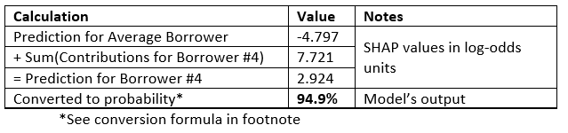
As mentioned earlier, one of the biggest reasons ML models don’t make it out of the lab and into production is that end users do not trust them. Suppose our end user, a loan officer, is running our model on a single borrower (borrower #4 in our dataset). The model predicts this borrower is 94.9% likely to default. Very risky. Before denying the application, the loan officer would like to know why the model dislikes this borrower so much. Using XAI, we can decompose the prediction into its components. There are several ways to visualize these components. My favorite is the decision plot, also from the SHAP package:

如前所述，机器学习模型无法在实验室中投入生产的最大原因之一是最终用户不信任它们。假设我们的最终用户(贷款人员)在单个借款人(数据集中的借款人4)上运行我们的模型。该模型预测该借款人违约的可能性为94.9％。风险很大。在拒绝申请之前，信贷员想知道为什么模型如此不喜欢该借款人。使用XAI，我们可以将预测分解为其组成部分。有几种方法可以可视化这些组件。我最喜欢的是决策图，也来自SHAP包：

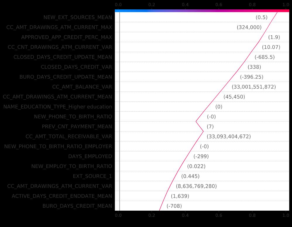
How should we read this chart?

我们应该如何阅读此图表？

· In this plot, we show the impact of the top 20 most important features on the model’s prediction for borrower #4.

·在此图中，我们显示了前20个最重要特征对模型对4号借款人的预测的影响。

· The prediction is the red line. The model’s output is where the line meets the color band at the top of the chart, 94.9% likely to default.

·预测是红线。模型的输出是线条与图表顶部的色带相交的地方，默认值是94.9％。

· Features that mark the borrower as riskier-than-average move the line to the right. Features that mark the borrower as safer-than-average move the line to the left.

·将借款人标记为风险高于平均水平的功能将行向右移动。将借款人标记为高于平均水平的功能将行向左移动。

· Feature values for borrower #4 are in gray, next to the line.

·借方＃4的特征值在该行旁边为灰色。

· Although it might be hard to see from the chart, not all features move the line to the same degree. Features on top move it more.

·尽管可能很难从图表中看到，但并非所有功能都将线移动到相同的程度。顶部的功能将其进一步移动。

What is it telling us?

它告诉我们什么？

· The borrower’s credit score is about average for our cohort, but

·借款人的信用评分大约是我们同类人群的平均水平，但

· Almost everything else about this borrower is a red flag. It’s not one thing: It’s everything.

·关于此借款人的几乎所有其他内容都是危险信号。这不是一回事：这就是一切。

So what?

所以呢？

· This should give the loan officer some confidence in the prediction. Even if the model is wrong about one or two features, the conclusion shouldn’t change much.

·这应该使信贷员对该预测有一定的信心。即使该模型关于一个或两个特征是错误的，结论也不会有太大变化。

If this were a production model, feature labels would be more user-friendly and the loan officer would be able to click on them to get additional information, such as how borrower #4 compares with the rest on any given feature, or the feature dependency plot shown earlier.

如果这是一种生产模型，则功能标签将更加易于使用，并且借贷人员将可以单击它们以获取其他信息，例如，借方＃4与其他任何给定功能的其余部分相比，或者功能依赖性前面显示的情节。

The only problem is that this plot doesn’t show our full model, only the top 20 features. Here is the underlying data:

唯一的问题是，该图不显示完整的模型，而仅显示前20个功能。以下是基础数据：

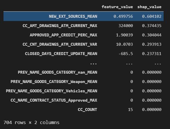
How should we read this chart?

我们应该如何阅读此图表？

· Each row represents a model feature, 704 in total.

·每行代表一个模型特征，总共704个。

· The middle column shows the feature’s value for borrower #4.

·中间一栏显示了4号借方的要素价值。

· The right column shows the feature’s contribution to the model’s prediction for borrower #4, denominated in log-odds units. The data is sorted by the absolute value of this column. This puts the most important features on top, just like in previous plots.

·右列显示了特征对第4号借款人的模型预测的贡献，以对数为单位。数据按此列的绝对值排序。就像以前的情节一样，这将最重要的功能放在首位。

· If we add up the right column to the model’s average prediction across all borrowers, we get the model’s prediction for borrower #4. Here’s the math:

·如果在所有借款人的模型平均预测中加右栏，则将得出4号借款人的模型预测。这是数学：

What is it telling us?

它告诉我们什么？

· Reading down the right column, this borrower’s credit score is significant, but almost every other feature contributes a little to the risky label. Lots of risk factors, no mitigants.

·在右列中读到该借款人的信用评分很重要，但是几乎所有其他功能都对风险标签有所贡献。风险因素很多，没有缓解措施。

· Looking at the bottom of the list, 336 of our 704 features have zero contribution, which means they do not affect our model’s prediction for borrower #4 at all.

·从列表的底部看，我们704个功能中的336个贡献为零，这意味着它们根本不影响我们对4号借款人的模型预测。

So what?

所以呢？

· If this were a common pattern across borrowers (and not just for borrower #4), we would want to prune these zero-impact features from the model.

·如果这是借款人之间的共同模式(而不仅仅是4号借款人)，我们希望从模型中修剪这些零影响功能。

3.审计师：管理风险，公平性和偏见 (3. Auditor: Manage Risk, Fairness and Bias)

Before a model goes to production, it will typically need to be validated by a separate team. Organizations call these teams by different names: model validation, model risk, AI governance or something similar. For simplicity, let’s call them the auditor.

模型投入生产之前，通常需要由单独的团队进行验证。组织用不同的名称称呼这些团队：模型验证，模型风险，AI治理或类似的东西。为简单起见，我们称他们为审核员。

The auditor is not concerned with a single prediction as above. They care about the model as a whole. For example, they may want to confirm that our (candidate) model is not biased against protected groups, which would be a violation of the Equal Credit Opportunity Act (if this model served US borrowers). Take gender, for example:

审核员并不关心上述单个预测。他们关心整个模型。例如，他们可能想要确认我们的(候选)模型不偏向受保护的群体，这将违反《平等信贷机会法》(如果该模型服务于美国借款人)。以性别为例：

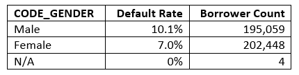
Our dataset includes about as many women as men and shows that women default less often. We would want to make sure that our model does not treat women unfairly by predicting they are more likely to default than men. This is simple to do: We simply compare predictions for men and women and use the t-test to see if the difference is significant.

我们的数据集包括大约和男性一样多的女性，并且表明女性违约的频率更低。我们希望通过预测女性比男性更容易违约，从而确保我们的模型不会不公平地对待女性。这很容易做到：我们只比较男性和女性的预测，然后使用t检验来检验差异是否显着。

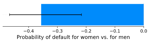
This chart shows the model tends to predict women will default less often, and the group difference is significant. This is consistent with our training data, summarized above. We can go further and test each feature separately:

此图显示该模型倾向于预测女性违约的频率会降低，并且群体差异非常明显。这与我们上面总结的训练数据一致。我们可以进一步测试每个功能：

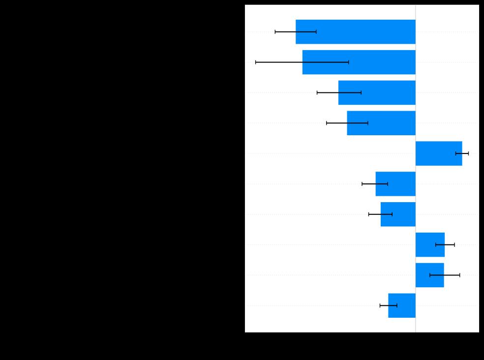
How should we read this chart?

我们应该如何阅读此图表？

· We once again look at the top 10 most important features.

·我们再次看一下最重要的十大功能。

· Features stretching to the left of the vertical line “favor” women and those to the right “favor” men.

·特征延伸到垂直线“喜欢”的女人的左边，延伸到右边“喜欢”的男人的女人。

· The plot also shows confidence intervals.

·该图还显示了置信区间。

What is this chart telling us?

这张图告诉我们什么？

· Most features favor women, consistent with the underlying distribution. This is good, since our model is not distorting things.

·大多数功能都偏爱女性，这与潜在的分布保持一致。这很好，因为我们的模型不会扭曲事物。

· Some features still favor men, such as the ratio between the annual loan payment and income. Possibly this is because men in our dataset have a higher income.

·一些功能仍然偏爱男性，例如年贷款额与收入之间的比率。这可能是因为我们数据集中的男性收入较高。

· We built this chart on a sample. We could probably get better (tighter) confidence intervals if we used a larger sample.

·我们将此图表建立在样本上。如果使用更大的样本，我们可能会获得更好(更紧)的置信区间。

So what?

所以呢？

· At this point, the auditor will consider this evidence to determine whether a model should move forward to production. Different lenders will react to the evidence in different ways. Some may kick out features that favor men, even though they may make the model less accurate. Others will accept all features provided they do not cross a certain significance threshold. Yet others may only look at the aggregate prediction.

·此时，审核员将考虑该证据，以确定模型是否应继续进行生产。不同的贷方将以不同的方式对证据做出React。有些人可能会推出一些偏爱男性的功能，即使它们可能会使模型的准确性降低。其他人将接受所有特征，只要它们没有超过特定的显着性阈值。还有一些人可能只看汇总预测。

The same analysis would be repeated for other protected groups — by race, age, sexual orientation, disability status, etc.

对于其他受保护群体，将按照种族，年龄，性取向，残疾状况等进行同样的分析。

结论 (Conclusion)

Explainable AI (XAI) is one of the most exciting areas of development in AI because it can facilitate conversations between modelers and domain experts that would otherwise not happen. These conversations are highly valuable because they get technical and business stakeholders on the same page. Together, we can make sure the model is “right for the right reasons” and maybe even solve our Cassandra problem.

可解释性AI(XAI)是AI开发中最令人兴奋的领域之一，因为它可以促进建模人员与领域专家之间的对话，而这种对话本来不会发生的。这些对话非常有价值，因为它们在同一页面上吸引了技术和业务利益相关者。在一起，我们可以确保模型“因正确的原因而正确”，甚至可以解决我们的Cassandra问题。