我在前面已经给出了模拟退火法的完整知识点和源码实现:智能优化算法—蚁群算法(Python实现)
模拟退火和蒙特卡洛实验一样,全局随机,由于没有自适应的过程(例如向最优靠近、权重梯度下降等),对于复杂函数寻优,很难会找到最优解,都是近似最优解;然而像蝙蝠算法、粒子群算法等有向最优逼近且通过最优最差调整参数的步骤,虽然对于下图函数易陷入局部最优,但是寻优精度相对较高。如果理解这段话应该就明白了为什么神经网络训练前如果初步寻优一组较好的网络参数,会使训练效果提高很多,也会更快达到误差精度。
#===========1导包================
import matplotlib.pyplot as plt
import pandas as pd
from sko.SA import SA

#============2定义问题===============
fun = lambda x: x[0] ** 2 + (x[1] - 0.05) ** 2 + x[2] ** 2

#=========3运行模拟退火算法===========
sa = SA(func=fun, x0=[1, 1, 1], T_max=1, T_min=1e-9, L=300, max_stay_counter=150)
best_x, best_y = sa.run()
print('best_x:', best_x, 'best_y', best_y)

#=======4画出结果=======
plt.plot(pd.DataFrame(sa.best_y_history).cummin(axis=0))
plt.show()


#scikit-opt 还提供了三种模拟退火流派: Fast, Boltzmann, Cauchy.

#===========1.1 Fast Simulated Annealing=====================
from sko.SA import SAFast

sa_fast = SAFast(func=demo_func, x0=[1, 1, 1], T_max=1, T_min=1e-9, q=0.99, L=300, max_stay_counter=150)
sa_fast.run()
print('Fast Simulated Annealing: best_x is ', sa_fast.best_x, 'best_y is ', sa_fast.best_y)

#===========1.2 Fast Simulated Annealing with bounds=====================
from sko.SA import SAFast

sa_fast = SAFast(func=demo_func, x0=[1, 1, 1], T_max=1, T_min=1e-9, q=0.99, L=300, max_stay_counter=150,
                 lb=[-1, 1, -1], ub=[2, 3, 4])
sa_fast.run()
print('Fast Simulated Annealing with bounds: best_x is ', sa_fast.best_x, 'best_y is ', sa_fast.best_y)

#===========2.1 Boltzmann Simulated Annealing====================
from sko.SA import SABoltzmann

sa_boltzmann = SABoltzmann(func=demo_func, x0=[1, 1, 1], T_max=1, T_min=1e-9, q=0.99, L=300, max_stay_counter=150)
sa_boltzmann.run()
print('Boltzmann Simulated Annealing: best_x is ', sa_boltzmann.best_x, 'best_y is ', sa_fast.best_y)

#===========2.2 Boltzmann Simulated Annealing with bounds====================
from sko.SA import SABoltzmann

sa_boltzmann = SABoltzmann(func=demo_func, x0=[1, 1, 1], T_max=1, T_min=1e-9, q=0.99, L=300, max_stay_counter=150,
                           lb=-1, ub=[2, 3, 4])
sa_boltzmann.run()
print('Boltzmann Simulated Annealing with bounds: best_x is ', sa_boltzmann.best_x, 'best_y is ', sa_fast.best_y)

#==================3.1 Cauchy Simulated Annealing==================
from sko.SA import SACauchy

sa_cauchy = SACauchy(func=demo_func, x0=[1, 1, 1], T_max=1, T_min=1e-9, q=0.99, L=300, max_stay_counter=150)
sa_cauchy.run()
print('Cauchy Simulated Annealing: best_x is ', sa_cauchy.best_x, 'best_y is ', sa_cauchy.best_y)

#==================3.2 Cauchy Simulated Annealing with bounds==================
from sko.SA import SACauchy

sa_cauchy = SACauchy(func=demo_func, x0=[1, 1, 1], T_max=1, T_min=1e-9, q=0.99, L=300, max_stay_counter=150,
                     lb=[-1, 1, -1], ub=[2, 3, 4])
sa_cauchy.run()
print('Cauchy Simulated Annealing with bounds: best_x is ', sa_cauchy.best_x, 'best_y is ', sa_cauchy.best_y)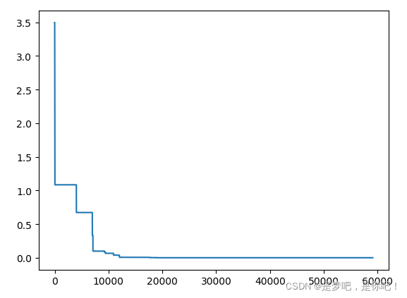
clear
clc
T=1000; %初始化温度值
T_min=1; %设置温度下界
alpha=0.99; %温度的下降率
num=1000; %颗粒总数
n=2; %自变量个数
sub=[-5,-5]; %自变量下限
up=[5,5]; %自变量上限
tu
for i=1:num
for j=1:n
x(i,j)=(up(j)-sub(j))*rand+sub(j);
end
fx(i,1)=fun(x(i,1),x(i,2));
end
%以最小化为例
[bestf,a]=min(fx);
bestx=x(a,:);
trace(1)=bestf;
while(T>T_min)
for i=1:num
for j=1:n
xx(i,j)=(up(j)-sub(j))*rand+sub(j);
end
ff(i,1)=fun(xx(i,1),xx(i,2));
delta=ff(i,1)-fx(i,1);
if delta<0
fx(i,1)=ff(i,1);
x(i,:)=xx(i,:);
else
P=exp(-delta/T);
if P>rand
fx(i,1)=ff(i,1);
x(i,:)=xx(i,:);
end
end
end
if min(fx)<bestf
[bestf,a]=min(fx);
bestx=x(a,:);
end
trace=[trace;bestf];
T=T*alpha;
end
disp('最优解为:')
disp(bestx)
disp('最优值为:')
disp(bestf)
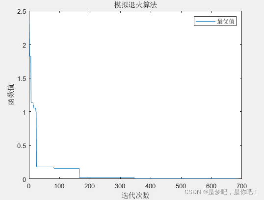
hold on
plot3(bestx(1),bestx(2),bestf,'ro','LineWidth',5)
figure
plot(trace)
xlabel('迭代次数')
ylabel('函数值')
title('模拟退火算法')
legend('最优值')function z=fun(x,y) z = x.^2 + y.^2 - 10*cos(2*pi*x) - 10*cos(2*pi*y) + 20;
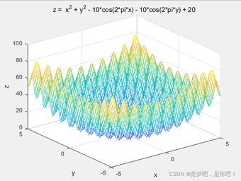
function tu
[x,y] = meshgrid(-5:0.1:5,-5:0.1:5);
z = x.^2 + y.^2 - 10*cos(2*pi*x) - 10*cos(2*pi*y) + 20;
figure
mesh(x,y,z)%建一个网格图,该网格图为三维曲面,有实色边颜色,无面颜色
hold on
xlabel('x')
ylabel('y')
zlabel('z')
title('z =  x^2 + y^2 - 10*cos(2*pi*x) - 10*cos(2*pi*y) + 20')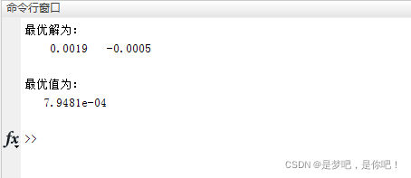
这里有一个待尝试的想法,先用蒙特卡洛/模拟退火迭代几次全局去找最优的区域,再通过其他有向最优逼近过程的算法再进一步寻优,或许会很大程度降低产生局部最优解的概率。
下面是模拟退火和蒙特卡洛对上述函数寻优的程序,迭代次数已设为一致,可以思考下两种程序写法的效率、共同点、缺点。理论研究讲究结果好,实际应用既要保证结果好也要保证程序运算效率。
clear
clc
num=689000; %颗粒总数
n=2; %自变量个数
sub=[-5,-5]; %自变量下限
up=[5,5]; %自变量上限
tu
x=zeros(num,n);
fx=zeros(num,1);
for i=1:num
for j=1:n
x(i,j)=(up(j)-sub(j))*rand+sub(j);
    end
    fx(i,1)=fun(x(i,1),x(i,2));
end

[bestf,a]=min(fx);
bestx=x(a,:);

disp('最优解为:')
disp(bestx)
disp('最优值为:')
disp(bestf)
hold on
plot3(bestx(1),bestx(2),bestf,'ro','LineWidth',5)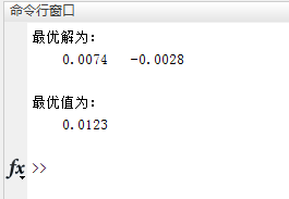
效果确实值得商榷。