RFBnet是SSD的一种加强版,主要是利用了膨胀卷积这一方法增大了感受野,相比于普通的ssd,RFBnet也是一种加强吧
RFBnet是改进版的SSD,其整体的结构与SSD相差不大,其主要特点是在SSD的特征提取网络上用了RFB模块。
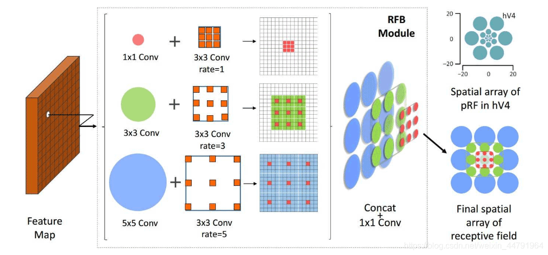
RFB的全称Receptive Field Block,是一种轻量级的、而且集成了各类检测算法优点的模块,结合了Inception、虫洞卷积的思想,以提高感受野的方式提高网络的特征提取能力。

RFBnet采用的主干网络是VGG网络,关于VGG的介绍大家可以看我的另外一篇博客https:,这里的VGG网络相比普通的VGG网络有一定的修改,主要修改的地方就是:
1、将VGG16的FC6和FC7层转化为卷积层。
2、增加了RFB模块。
主要使用到的RFB模块有两种,一种是BasicRFB,另一种是BasicRFB_a。
二者使用的思想相同,构造有些许不同。
BasicRFB的结构如下:
BasicRFB_a和BasicRFB类似,并联结构增加,有8个并联。
实现代码:
from keras.layers import (Activation, BatchNormalization, Conv2D, Lambda,
MaxPooling2D, UpSampling2D, concatenate)
def conv2d_bn(x,filters,num_row,num_col,padding='same',stride=1,dilation_rate=1,relu=True):
x = Conv2D(
filters, (num_row, num_col),
strides=(stride,stride),
padding=padding,
dilation_rate=(dilation_rate, dilation_rate),
use_bias=False)(x)
x = BatchNormalization()(x)
if relu:
x = Activation("relu")(x)
return x
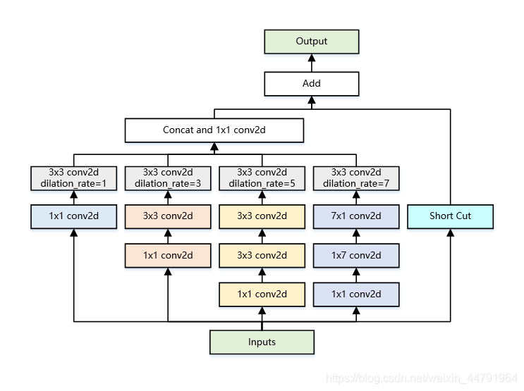
def BasicRFB(x,input_filters,output_filters,stride=1,map_reduce=8):
#-------------------------------------------------------#
# BasicRFB模块是一个残差结构
# 主干部分使用不同膨胀率的卷积进行特征提取
# 残差边只包含一个调整宽高和通道的1x1卷积
#-------------------------------------------------------#
input_filters_div = input_filters//map_reduce
branch_0 = conv2d_bn(x, input_filters_div*2, 1, 1, stride=stride)
branch_0 = conv2d_bn(branch_0, input_filters_div*2, 3, 3, relu=False)
branch_1 = conv2d_bn(x, input_filters_div, 1, 1)
branch_1 = conv2d_bn(branch_1, input_filters_div*2, 3, 3, stride=stride)
branch_1 = conv2d_bn(branch_1, input_filters_div*2, 3, 3, dilation_rate=3, relu=False)
branch_2 = conv2d_bn(x, input_filters_div, 1, 1)
branch_2 = conv2d_bn(branch_2, (input_filters_div//2)*3, 3, 3)
branch_2 = conv2d_bn(branch_2, input_filters_div*2, 3, 3, stride=stride)
branch_2 = conv2d_bn(branch_2, input_filters_div*2, 3, 3, dilation_rate=5, relu=False)
branch_3 = conv2d_bn(x, input_filters_div, 1, 1)
branch_3 = conv2d_bn(branch_3, (input_filters_div//2)*3, 1, 7)
branch_3 = conv2d_bn(branch_3, input_filters_div*2, 7, 1, stride=stride)
branch_3 = conv2d_bn(branch_3, input_filters_div*2, 3, 3, dilation_rate=7, relu=False)
#-------------------------------------------------------#
# 将不同膨胀率的卷积结果进行堆叠
# 利用1x1卷积调整通道数
#-------------------------------------------------------#
out = concatenate([branch_0,branch_1,branch_2,branch_3],axis=-1)
out = conv2d_bn(out, output_filters, 1, 1, relu=False)
#-------------------------------------------------------#
# 残差边也需要卷积,才可以相加
#-------------------------------------------------------#
short = conv2d_bn(x, output_filters, 1, 1, stride=stride, relu=False)
out = Lambda(lambda x: x[0] + x[1])([out,short])
out = Activation("relu")(out)
return out
def BasicRFB_a(x, input_filters, output_filters, stride=1, map_reduce=8):
#-------------------------------------------------------#
# BasicRFB_a模块也是一个残差结构
# 主干部分使用不同膨胀率的卷积进行特征提取
# 残差边只包含一个调整宽高和通道的1x1卷积
#-------------------------------------------------------#
input_filters_div = input_filters//map_reduce
branch_0 = conv2d_bn(x,input_filters_div,1,1,stride=stride)
branch_0 = conv2d_bn(branch_0,input_filters_div,3,3,relu=False)
branch_1 = conv2d_bn(x,input_filters_div,1,1)
branch_1 = conv2d_bn(branch_1,input_filters_div,3,1,stride=stride)
branch_1 = conv2d_bn(branch_1,input_filters_div,3,3,dilation_rate=3,relu=False)
branch_2 = conv2d_bn(x,input_filters_div,1,1)
branch_2 = conv2d_bn(branch_2,input_filters_div,1,3,stride=stride)
branch_2 = conv2d_bn(branch_2,input_filters_div,3,3,dilation_rate=3,relu=False)
branch_3 = conv2d_bn(x,input_filters_div,1,1)
branch_3 = conv2d_bn(branch_3,input_filters_div,3,1,stride=stride)
branch_3 = conv2d_bn(branch_3,input_filters_div,3,3,dilation_rate=5,relu=False)
branch_4 = conv2d_bn(x,input_filters_div,1,1)
branch_4 = conv2d_bn(branch_4,input_filters_div,1,3,stride=stride)
branch_4 = conv2d_bn(branch_4,input_filters_div,3,3,dilation_rate=5,relu=False)
branch_5 = conv2d_bn(x,input_filters_div//2,1,1)
branch_5 = conv2d_bn(branch_5,(input_filters_div//4)*3,1,3)
branch_5 = conv2d_bn(branch_5,input_filters_div,3,1,stride=stride)
branch_5 = conv2d_bn(branch_5,input_filters_div,3,3,dilation_rate=7,relu=False)
branch_6 = conv2d_bn(x,input_filters_div//2,1,1)
branch_6 = conv2d_bn(branch_6,(input_filters_div//4)*3,3,1)
branch_6 = conv2d_bn(branch_6,input_filters_div,1,3,stride=stride)
branch_6 = conv2d_bn(branch_6,input_filters_div,3,3,dilation_rate=7,relu=False)
#-------------------------------------------------------#
# 将不同膨胀率的卷积结果进行堆叠
# 利用1x1卷积调整通道数
#-------------------------------------------------------#
out = concatenate([branch_0,branch_1,branch_2,branch_3,branch_4,branch_5,branch_6],axis=-1)
out = conv2d_bn(out, output_filters, 1, 1, relu=False)
#-------------------------------------------------------#
# 残差边也需要卷积,才可以相加
#-------------------------------------------------------#
short = conv2d_bn(x, output_filters, 1, 1, stride=stride, relu=False)
out = Lambda(lambda x: x[0] + x[1])([out, short])
out = Activation("relu")(out)
return out
#--------------------------------#
# 取Conv4_3和fc7进行特征融合
#--------------------------------#
def Normalize(net):
# 38,38,512 -> 38,38,256
branch_0 = conv2d_bn(net["conv4_3"], 256, 1, 1)
# 19,19,512 -> 38,38,256
branch_1 = conv2d_bn(net['fc7'], 256, 1, 1)
branch_1 = UpSampling2D()(branch_1)
# 38,38,256 + 38,38,256 -> 38,38,512
out = concatenate([branch_0,branch_1],axis=-1)
# 38,38,512 -> 38,38,512
out = BasicRFB_a(out,512,512)
return out
def backbone(input_tensor):
#----------------------------主干特征提取网络开始---------------------------#
# RFB结构,net字典
net = {}
# Block 1
net['input'] = input_tensor
# 300,300,3 -> 150,150,64
net['conv1_1'] = Conv2D(64, kernel_size=(3,3),
activation='relu',
padding='same',
name='conv1_1')(net['input'])
net['conv1_2'] = Conv2D(64, kernel_size=(3,3),
activation='relu',
padding='same',
name='conv1_2')(net['conv1_1'])
net['pool1'] = MaxPooling2D((2, 2), strides=(2, 2), padding='same',
name='pool1')(net['conv1_2'])
# Block 2
# 150,150,64 -> 75,75,128
net['conv2_1'] = Conv2D(128, kernel_size=(3,3),
activation='relu',
padding='same',
name='conv2_1')(net['pool1'])
net['conv2_2'] = Conv2D(128, kernel_size=(3,3),
activation='relu',
padding='same',
name='conv2_2')(net['conv2_1'])
net['pool2'] = MaxPooling2D((2, 2), strides=(2, 2), padding='same',
name='pool2')(net['conv2_2'])
# Block 3
# 75,75,128 -> 38,38,256
net['conv3_1'] = Conv2D(256, kernel_size=(3,3),
activation='relu',
padding='same',
name='conv3_1')(net['pool2'])
net['conv3_2'] = Conv2D(256, kernel_size=(3,3),
activation='relu',
padding='same',
name='conv3_2')(net['conv3_1'])
net['conv3_3'] = Conv2D(256, kernel_size=(3,3),
activation='relu',
padding='same',
name='conv3_3')(net['conv3_2'])
net['pool3'] = MaxPooling2D((2, 2), strides=(2, 2), padding='same',
name='pool3')(net['conv3_3'])
# Block 4
# 38,38,256 -> 19,19,512
net['conv4_1'] = Conv2D(512, kernel_size=(3,3),
activation='relu',
padding='same',
name='conv4_1')(net['pool3'])
net['conv4_2'] = Conv2D(512, kernel_size=(3,3),
activation='relu',
padding='same',
name='conv4_2')(net['conv4_1'])
net['conv4_3'] = Conv2D(512, kernel_size=(3,3),
activation='relu',
padding='same',
name='conv4_3')(net['conv4_2'])
net['pool4'] = MaxPooling2D((2, 2), strides=(2, 2), padding='same',
name='pool4')(net['conv4_3'])
# Block 5
# 19,19,512 -> 19,19,512
net['conv5_1'] = Conv2D(512, kernel_size=(3,3),
activation='relu',
padding='same',
name='conv5_1')(net['pool4'])
net['conv5_2'] = Conv2D(512, kernel_size=(3,3),
activation='relu',
padding='same',
name='conv5_2')(net['conv5_1'])
net['conv5_3'] = Conv2D(512, kernel_size=(3,3),
activation='relu',
padding='same',
name='conv5_3')(net['conv5_2'])
net['pool5'] = MaxPooling2D((3, 3), strides=(1, 1), padding='same',
name='pool5')(net['conv5_3'])
# FC6
# 19,19,512 -> 19,19,1024
net['fc6'] = Conv2D(1024, kernel_size=(3,3), dilation_rate=(6, 6),
activation='relu', padding='same',
name='fc6')(net['pool5'])
# x = Dropout(0.5, name='drop6')(x)
# FC7
# 19,19,1024 -> 19,19,1024
net['fc7'] = Conv2D(1024, kernel_size=(1,1), activation='relu',
padding='same', name='fc7')(net['fc6'])
#----------------------------------------------------------#
# conv4_3 38,38,512 -> 38,38,512 net['norm']
# fc7 19,19,1024 ->
#----------------------------------------------------------#
net['norm'] = Normalize(net)
# 19,19,1024 -> 19,19,1024
net['rfb_1'] = BasicRFB(net['fc7'],1024,1024)
# 19,19,1024 -> 10,10,512
net['rfb_2'] = BasicRFB(net['rfb_1'],1024,512,stride=2)
# 10,10,512 -> 5,5,256
net['rfb_3'] = BasicRFB(net['rfb_2'],512,256,stride=2)
# 5,5,256 -> 5,5,128
net['conv6_1'] = conv2d_bn(net['rfb_3'],128,1,1)
# 5,5,128 -> 3,3,256
net['conv6_2'] = conv2d_bn(net['conv6_1'],256,3,3,padding="valid")
# 3,3,256 -> 3,3,128
net['conv7_1'] = conv2d_bn(net['conv6_2'],128,1,1)
# 3,3,128 -> 1,1,256
net['conv7_2'] = conv2d_bn(net['conv7_1'],256,3,3,padding="valid")
return net
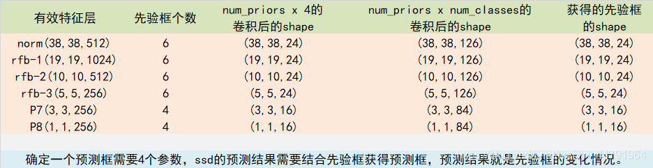
由上图我们可以知道,我们取conv4的第三次卷积的特征、fc7的特征进行组合后经过一个BasicRFB_a获得P3作为有效特征层、还有上图的P4、P5、P6、P7、P8作为有效特征层,为了和普通特征层区分,我们称之为有效特征层,来获取预测结果。
对获取到的每一个有效特征层,我们分别对其进行一次num_anchors x 4的卷积、一次num_anchors x num_classes的卷积。而num_anchors指的是该特征层所拥有的先验框数量。
其中:num_anchors x 4的卷积 用于预测 该特征层上 每一个网格点上 每一个先验框的变化情况。(为什么说是变化情况呢,这是因为ssd的预测结果需要结合先验框获得预测框,预测结果就是先验框的变化情况。)
num_anchors x num_classes的卷积 用于预测 该特征层上 每一个网格点上 每一个预测框对应的种类。
每一个有效特征层对应的先验框对应着该特征层上 每一个网格点上 预先设定好的三个框。
所有的特征层对应的预测结果的shape如下:
实现代码为:
from keras.layers import (Activation, Concatenate, Conv2D, Flatten, Input,
                          Reshape)
from keras.models import Model
from nets.backbone import backbone
def RFB300(input_shape, num_classes=21):
    #---------------------------------#
    #   典型的输入大小为[300,300,3]
    #---------------------------------#
    input_tensor = Input(shape=input_shape)
    # net变量里面包含了整个RFB的结构,通过层名可以找到对应的特征层
    net = backbone(input_tensor)
    #-----------------------将提取到的主干特征进行处理---------------------------#
    # 对conv4_3的通道进行l2标准化处理
    # 38,38,512
    num_anchors = 6
    # 预测框的处理
    # num_anchors表示每个网格点先验框的数量,4是x,y,h,w的调整
    net['norm_mbox_loc']        = Conv2D(num_anchors * 4, kernel_size=(3,3), padding='same', name='norm_mbox_loc')(net['norm'])
    net['norm_mbox_loc_flat']   = Flatten(name='norm_mbox_loc_flat')(net['norm_mbox_loc'])
    # num_anchors表示每个网格点先验框的数量,num_classes是所分的类
    net['norm_mbox_conf']       = Conv2D(num_anchors * num_classes, kernel_size=(3,3), padding='same',name='norm_mbox_conf')(net['norm'])
    net['norm_mbox_conf_flat']  = Flatten(name='norm_mbox_conf_flat')(net['norm_mbox_conf'])
    # 对rfb_1层进行处理
    # 19,19,1024
    num_anchors = 6
    # 预测框的处理
    # num_anchors表示每个网格点先验框的数量,4是x,y,h,w的调整
    net['rfb_1_mbox_loc']       = Conv2D(num_anchors * 4, kernel_size=(3,3),padding='same',name='rfb_1_mbox_loc')(net['rfb_1'])
    net['rfb_1_mbox_loc_flat']  = Flatten(name='rfb_1_mbox_loc_flat')(net['rfb_1_mbox_loc'])
    # num_anchors表示每个网格点先验框的数量,num_classes是所分的类
    net['rfb_1_mbox_conf']      = Conv2D(num_anchors * num_classes, kernel_size=(3,3),padding='same',name='rfb_1_mbox_conf')(net['rfb_1'])
    net['rfb_1_mbox_conf_flat'] = Flatten(name='rfb_1_mbox_conf_flat')(net['rfb_1_mbox_conf'])
    # 对rfb_2进行处理
    # 10,10,512
    num_anchors = 6
    # 预测框的处理
    # num_anchors表示每个网格点先验框的数量,4是x,y,h,w的调整
    net['rfb_2_mbox_loc']       = Conv2D(num_anchors * 4, kernel_size=(3,3), padding='same',name='rfb_2_mbox_loc')(net['rfb_2'])
    net['rfb_2_mbox_loc_flat']  = Flatten(name='rfb_2_mbox_loc_flat')(net['rfb_2_mbox_loc'])
    # num_anchors表示每个网格点先验框的数量,num_classes是所分的类
    net['rfb_2_mbox_conf']      = Conv2D(num_anchors * num_classes, kernel_size=(3,3), padding='same',name='rfb_2_mbox_conf')(net['rfb_2'])
    net['rfb_2_mbox_conf_flat'] = Flatten(name='rfb_2_mbox_conf_flat')(net['rfb_2_mbox_conf'])
    # 对rfb_3进行处理
    # 5,5,256
    num_anchors = 6
    # 预测框的处理
    # num_anchors表示每个网格点先验框的数量,4是x,y,h,w的调整
    net['rfb_3_mbox_loc']       = Conv2D(num_anchors * 4, kernel_size=(3,3), padding='same',name='rfb_3_mbox_loc')(net['rfb_3'])
    net['rfb_3_mbox_loc_flat']  = Flatten(name='rfb_3_mbox_loc_flat')(net['rfb_3_mbox_loc'])
    # num_anchors表示每个网格点先验框的数量,num_classes是所分的类
    net['rfb_3_mbox_conf']      = Conv2D(num_anchors * num_classes, kernel_size=(3,3), padding='same',name='rfb_3_mbox_conf')(net['rfb_3'])
    net['rfb_3_mbox_conf_flat'] = Flatten(name='rfb_3_mbox_conf_flat')(net['rfb_3_mbox_conf'])
    # 对conv6_2进行处理
    # 3,3,256
    num_anchors = 4
    # 预测框的处理
    # num_anchors表示每个网格点先验框的数量,4是x,y,h,w的调整
    net['conv6_2_mbox_loc']         = Conv2D(num_anchors * 4, kernel_size=(3,3), padding='same',name='conv6_2_mbox_loc')(net['conv6_2'])
    net['conv6_2_mbox_loc_flat']    = Flatten(name='conv6_2_mbox_loc_flat')(net['conv6_2_mbox_loc'])
    # num_anchors表示每个网格点先验框的数量,num_classes是所分的类
    net['conv6_2_mbox_conf']        = Conv2D(num_anchors * num_classes, kernel_size=(3,3), padding='same',name='conv6_2_mbox_conf')(net['conv6_2'])
    net['conv6_2_mbox_conf_flat']   = Flatten(name='conv6_2_mbox_conf_flat')(net['conv6_2_mbox_conf'])
    # 对conv7_2进行处理
    # 1,1,256
    num_anchors = 4
    # 预测框的处理
    # num_anchors表示每个网格点先验框的数量,4是x,y,h,w的调整
    net['conv7_2_mbox_loc']         = Conv2D(num_anchors * 4, kernel_size=(3,3), padding='same',name='conv7_2_mbox_loc')(net['conv7_2'])
    net['conv7_2_mbox_loc_flat']    = Flatten(name='conv7_2_mbox_loc_flat')(net['conv7_2_mbox_loc'])
    # num_anchors表示每个网格点先验框的数量,num_classes是所分的类
    net['conv7_2_mbox_conf']        = Conv2D(num_anchors * num_classes, kernel_size=(3,3), padding='same',name='conv7_2_mbox_conf')(net['conv7_2'])
    net['conv7_2_mbox_conf_flat']   = Flatten(name='conv7_2_mbox_conf_flat')(net['conv7_2_mbox_conf'])
    # 将所有结果进行堆叠
    net['mbox_loc'] = Concatenate(axis=1, name='mbox_loc')([net['norm_mbox_loc_flat'],
                                                            net['rfb_1_mbox_loc_flat'],
                                                            net['rfb_2_mbox_loc_flat'],
                                                            net['rfb_3_mbox_loc_flat'],
                                                            net['conv6_2_mbox_loc_flat'],
                                                            net['conv7_2_mbox_loc_flat']])
    net['mbox_conf'] = Concatenate(axis=1, name='mbox_conf')([net['norm_mbox_conf_flat'],
                                                            net['rfb_1_mbox_conf_flat'],
                                                            net['rfb_2_mbox_conf_flat'],
                                                            net['rfb_3_mbox_conf_flat'],
                                                            net['conv6_2_mbox_conf_flat'],
                                                            net['conv7_2_mbox_conf_flat']])
    # 11620,4
    net['mbox_loc']     = Reshape((-1, 4), name='mbox_loc_final')(net['mbox_loc'])
    # 11620,21
    net['mbox_conf']    = Reshape((-1, num_classes), name='mbox_conf_logits')(net['mbox_conf'])
    net['mbox_conf']    = Activation('softmax', name='mbox_conf_final')(net['mbox_conf'])
    # 11620,25
    net['predictions']  = Concatenate(axis =-1, name='predictions')([net['mbox_loc'], net['mbox_conf']])
    model = Model(net['input'], net['predictions'])
    return model
我们通过对每一个特征层的处理,可以获得三个内容,分别是:
num_anchors x 4的卷积 用于预测 该特征层上 每一个网格点上 每一个先验框的变化情况。**
num_anchors x num_classes的卷积 用于预测 该特征层上 每一个网格点上 每一个预测框对应的种类。
每一个有效特征层对应的先验框对应着该特征层上 每一个网格点上 预先设定好的多个框。
我们利用 num_anchors x 4的卷积 与 每一个有效特征层对应的先验框 获得框的真实位置。
每一个有效特征层对应的先验框就是,如图所示的作用:
每一个有效特征层将整个图片分成与其长宽对应的网格,如conv4-3和fl7组合成的特征层就是将整个图像分成38x38个网格;然后从每个网格中心建立多个先验框,如conv4-3和fl7组合成的有效特征层就是建立了6个先验框;
对于conv4-3和fl7组合成的特征层来讲,整个图片被分成38x38个网格,每个网格中心对应6个先验框,一共包含了,38x38x6个,8664个先验框。

先验框虽然可以代表一定的框的位置信息与框的大小信息,但是其是有限的,无法表示任意情况,因此还需要调整,RFBnet利用num_anchors x 4的卷积的结果对先验框进行调整。
num_anchors x 4中的num_anchors表示了这个网格点所包含的先验框数量,其中的4表示了x_offset、y_offset、h和w的调整情况。
x_offset与y_offset代表了真实框距离先验框中心的xy轴偏移情况。h和w代表了真实框的宽与高相对于先验框的变化情况。
RFBnet解码过程就是将每个网格的中心点加上它对应的x_offset和y_offset,加完后的结果就是预测框的中心,然后再利用 先验框和h、w结合 计算出预测框的长和宽。这样就能得到整个预测框的位置了。
当然得到最终的预测结构后还要进行得分排序与非极大抑制筛选这一部分基本上是所有目标检测通用的部分。
1、取出每一类得分大于self.obj_threshold的框和得分。
2、利用框的位置和得分进行非极大抑制。
实现代码如下:
def decode_boxes(self, mbox_loc, anchors, variances):
    # 获得先验框的宽与高
    anchor_width     = anchors[:, 2] - anchors[:, 0]
    anchor_height    = anchors[:, 3] - anchors[:, 1]
    # 获得先验框的中心点
    anchor_center_x  = 0.5 * (anchors[:, 2] + anchors[:, 0])
    anchor_center_y  = 0.5 * (anchors[:, 3] + anchors[:, 1])
    # 真实框距离先验框中心的xy轴偏移情况
    decode_bbox_center_x = mbox_loc[:, 0] * anchor_width * variances[0]
    decode_bbox_center_x += anchor_center_x
    decode_bbox_center_y = mbox_loc[:, 1] * anchor_height * variances[1]
    decode_bbox_center_y += anchor_center_y
    # 真实框的宽与高的求取
    decode_bbox_width   = np.exp(mbox_loc[:, 2] * variances[2])
    decode_bbox_width   *= anchor_width
    decode_bbox_height  = np.exp(mbox_loc[:, 3] * variances[3])
    decode_bbox_height  *= anchor_height
    # 获取真实框的左上角与右下角
    decode_bbox_xmin = decode_bbox_center_x - 0.5 * decode_bbox_width
    decode_bbox_ymin = decode_bbox_center_y - 0.5 * decode_bbox_height
    decode_bbox_xmax = decode_bbox_center_x + 0.5 * decode_bbox_width
    decode_bbox_ymax = decode_bbox_center_y + 0.5 * decode_bbox_height
    # 真实框的左上角与右下角进行堆叠
    decode_bbox = np.concatenate((decode_bbox_xmin[:, None],
                                    decode_bbox_ymin[:, None],
                                    decode_bbox_xmax[:, None],
                                    decode_bbox_ymax[:, None]), axis=-1)
    # 防止超出0与1
    decode_bbox = np.minimum(np.maximum(decode_bbox, 0.0), 1.0)
    return decode_bbox
def decode_box(self, predictions, anchors, image_shape, input_shape, letterbox_image, variances = [0.1, 0.1, 0.2, 0.2], confidence=0.5):
    #---------------------------------------------------#
    #   :4是回归预测结果
    #---------------------------------------------------#
    mbox_loc        = predictions[:, :, :4]
    #---------------------------------------------------#
    #   获得种类的置信度
    #---------------------------------------------------#
    mbox_conf       = predictions[:, :, 4:]
    results = []
    #----------------------------------------------------------------------------------------------------------------#
    #   对每一张图片进行处理,由于在predict.py的时候,我们只输入一张图片,所以for i in range(len(mbox_loc))只进行一次
    #----------------------------------------------------------------------------------------------------------------#
    for i in range(len(mbox_loc)):
        results.append([])
        #--------------------------------#
        #   利用回归结果对先验框进行解码
        #--------------------------------#
        decode_bbox = self.decode_boxes(mbox_loc[i], anchors, variances)
        for c in range(1, self.num_classes):
            #--------------------------------#
            #   取出属于该类的所有框的置信度
            #   判断是否大于门限
            #--------------------------------#
            c_confs     = mbox_conf[i, :, c]
            c_confs_m   = c_confs > confidence
            if len(c_confs[c_confs_m]) > 0:
                #-----------------------------------------#
                #   取出得分高于confidence的框
                #-----------------------------------------#
                boxes_to_process = decode_bbox[c_confs_m]
                confs_to_process = c_confs[c_confs_m]
                #-----------------------------------------#
                #   进行iou的非极大抑制
                #-----------------------------------------#
                idx         = self.sess.run(self.nms, feed_dict={self.boxes: boxes_to_process, self.scores: confs_to_process})
                #-----------------------------------------#
                #   取出在非极大抑制中效果较好的内容
                #-----------------------------------------#
                good_boxes  = boxes_to_process[idx]
                confs       = confs_to_process[idx][:, None]
                labels      = (c - 1) * np.ones((len(idx), 1))
                #-----------------------------------------#
                #   将label、置信度、框的位置进行堆叠。
                #-----------------------------------------#
                c_pred      = np.concatenate((good_boxes, labels, confs), axis=1)
                # 添加进result里
                results[-1].extend(c_pred)
        if len(results[-1]) > 0:
            results[-1] = np.array(results[-1])
            box_xy, box_wh = (results[-1][:, 0:2] + results[-1][:, 2:4])/2, results[-1][:, 2:4] - results[-1][:, 0:2]
            results[-1][:, :4] = self.ssd_correct_boxes(box_xy, box_wh, input_shape, image_shape, letterbox_image)
    return results
通过第三步,我们可以获得预测框在原图上的位置,而且这些预测框都是经过筛选的。这些筛选后的框可以直接绘制在图片上,就可以获得结果了。
从预测部分我们知道,每个特征层的预测结果,num_anchors x 4的卷积 用于预测 该特征层上 每一个网格点上 每一个先验框的变化情况。
也就是说,我们直接利用ssd网络预测到的结果,并不是预测框在图片上的真实位置,需要解码才能得到真实位置。
而在训练的时候,我们需要计算loss函数,这个loss函数是相对于RFB网络的预测结果的。我们需要把图片输入到当前的RFB网络中,得到预测结果;同时还需要把真实框的信息,进行编码,这个编码是把真实框的位置信息格式转化为RFB预测结果的格式信息。
也就是,我们需要找到 每一张用于训练的图片的每一个真实框对应的先验框,并求出如果想要得到这样一个真实框,我们的预测结果应该是怎么样的。
从预测结果获得真实框的过程被称作解码,而从真实框获得预测结果的过程就是编码的过程。
因此我们只需要将解码过程逆过来就是编码过程了。
实现代码如下:
def encode_box(self, box, return_iou=True, variances = [0.1, 0.1, 0.2, 0.2]):
    #---------------------------------------------#
    #   计算当前真实框和先验框的重合情况
    #   iou [self.num_anchors]
    #   encoded_box [self.num_anchors, 5]
    #---------------------------------------------#
    iou = self.iou(box)
    encoded_box = np.zeros((self.num_anchors, 4 + return_iou))
    #---------------------------------------------#
    #   找到每一个真实框,重合程度较高的先验框
    #   真实框可以由这个先验框来负责预测
    #---------------------------------------------#
    assign_mask = iou > self.overlap_threshold
    #---------------------------------------------#
    #   如果没有一个先验框重合度大于self.overlap_threshold
    #   则选择重合度最大的为正样本
    #---------------------------------------------#
    if not assign_mask.any():
        assign_mask[iou.argmax()] = True
    #---------------------------------------------#
    #   利用iou进行赋值
    #---------------------------------------------#
    if return_iou:
        encoded_box[:, -1][assign_mask] = iou[assign_mask]
    #---------------------------------------------#
    #   找到对应的先验框
    #---------------------------------------------#
    assigned_anchors = self.anchors[assign_mask]
    #---------------------------------------------#
    #   逆向编码,将真实框转化为rfb预测结果的格式
    #   先计算真实框的中心与长宽
    #---------------------------------------------#
    box_center  = 0.5 * (box[:2] + box[2:])
    box_wh      = box[2:] - box[:2]
    #---------------------------------------------#
    #   再计算重合度较高的先验框的中心与长宽
    #---------------------------------------------#
    assigned_anchors_center = (assigned_anchors[:, 0:2] + assigned_anchors[:, 2:4]) * 0.5
    assigned_anchors_wh     = (assigned_anchors[:, 2:4] - assigned_anchors[:, 0:2])
    #------------------------------------------------#
    #   逆向求取rfb应该有的预测结果
    #   先求取中心的预测结果,再求取宽高的预测结果
    #   存在改变数量级的参数,默认为[0.1,0.1,0.2,0.2]
    #------------------------------------------------#
    encoded_box[:, :2][assign_mask] = box_center - assigned_anchors_center
    encoded_box[:, :2][assign_mask] /= assigned_anchors_wh
    encoded_box[:, :2][assign_mask] /= np.array(variances)[:2]
    encoded_box[:, 2:4][assign_mask] = np.log(box_wh / assigned_anchors_wh)
    encoded_box[:, 2:4][assign_mask] /= np.array(variances)[2:4]
    return encoded_box.ravel()
利用上述代码我们可以获得,真实框对应的所有的iou较大先验框,并计算了真实框对应的所有iou较大的先验框应该有的预测结果。
在训练的时候我们只需要选择iou最大的先验框就行了,这个iou最大的先验框就是我们用来预测这个真实框所用的先验框。
因此我们还要经过一次筛选,将上述代码获得的真实框对应的所有的iou较大先验框的预测结果中,iou最大的那个筛选出来。
通过assign_boxes我们就获得了,输入进来的这张图片,应该有的预测结果是什么样子的。
实现代码如下:
def assign_boxes(self, boxes):
    #---------------------------------------------------#
    #   assignment分为3个部分
    #   :4      的内容为网络应该有的回归预测结果
    #   4:-1    的内容为先验框所对应的种类,默认为背景
    #   -1      的内容为当前先验框是否包含目标
    #---------------------------------------------------#
    assignment          = np.zeros((self.num_anchors, 4 + self.num_classes + 1))
    assignment[:, 4]    = 1.0
    if len(boxes) == 0:
        return assignment
    # 对每一个真实框都进行iou计算
    encoded_boxes   = np.apply_along_axis(self.encode_box, 1, boxes[:, :4])
    #---------------------------------------------------#
    #   在reshape后,获得的encoded_boxes的shape为:
    #   [num_true_box, num_anchors, 4 + 1]
    #   4是编码后的结果,1为iou
    #---------------------------------------------------#
    encoded_boxes   = encoded_boxes.reshape(-1, self.num_anchors, 5)
    #---------------------------------------------------#
    #   [num_anchors]求取每一个先验框重合度最大的真实框
    #---------------------------------------------------#
    best_iou        = encoded_boxes[:, :, -1].max(axis=0)
    best_iou_idx    = encoded_boxes[:, :, -1].argmax(axis=0)
    best_iou_mask   = best_iou > 0
    best_iou_idx    = best_iou_idx[best_iou_mask]
    #---------------------------------------------------#
    #   计算一共有多少先验框满足需求
    #---------------------------------------------------#
    assign_num      = len(best_iou_idx)
    # 将编码后的真实框取出
    encoded_boxes   = encoded_boxes[:, best_iou_mask, :]
    #---------------------------------------------------#
    #   编码后的真实框的赋值
    #---------------------------------------------------#
    assignment[:, :4][best_iou_mask] = encoded_boxes[best_iou_idx,np.arange(assign_num),:4]
    #----------------------------------------------------------#
    #   4代表为背景的概率,设定为0,因为这些先验框有对应的物体
    #----------------------------------------------------------#
    assignment[:, 4][best_iou_mask]     = 0
    assignment[:, 5:-1][best_iou_mask]  = boxes[best_iou_idx, 4:]
    #----------------------------------------------------------#
    #   -1表示先验框是否有对应的物体
    #----------------------------------------------------------#
    assignment[:, -1][best_iou_mask]    = 1
    # 通过assign_boxes我们就获得了,输入进来的这张图片,应该有的预测结果是什么样子的
    return assignment
loss的计算分为三个部分:
1、获取所有正标签的框的预测结果的回归loss。
2、获取所有正标签的种类的预测结果的交叉熵loss。
3、获取一定负标签的种类的预测结果的交叉熵loss。
由于在RFBnet的训练过程中,正负样本极其不平衡,即 存在对应真实框的先验框可能只有十来个,但是不存在对应真实框的负样本却有几千个,这就会导致负样本的loss值极大,因此我们可以考虑减少负样本的选取,对于ssd的训练来讲,常见的情况是取三倍正样本数量的负样本用于训练。这个三倍呢,也可以修改,调整成自己喜欢的数字。
实现代码如下:
import tensorflow as tf
class MultiboxLoss(object):
    def __init__(self, num_classes, alpha=1.0, neg_pos_ratio=3.0,
                 background_label_id=0, negatives_for_hard=100.0):
        self.num_classes = num_classes
        self.alpha = alpha
        self.neg_pos_ratio = neg_pos_ratio
        if background_label_id != 0:
            raise Exception('Only 0 as background label id is supported')
        self.background_label_id = background_label_id
        self.negatives_for_hard = negatives_for_hard
    def _l1_smooth_loss(self, y_true, y_pred):
        abs_loss = tf.abs(y_true - y_pred)
        sq_loss = 0.5 * (y_true - y_pred)**2
        l1_loss = tf.where(tf.less(abs_loss, 1.0), sq_loss, abs_loss - 0.5)
        return tf.reduce_sum(l1_loss, -1)
    def _softmax_loss(self, y_true, y_pred):
        y_pred = tf.maximum(y_pred, 1e-7)
        softmax_loss = -tf.reduce_sum(y_true * tf.log(y_pred),
                                      axis=-1)
        return softmax_loss
    def compute_loss(self, y_true, y_pred):
        # --------------------------------------------- #
        #   y_true batch_size, 11620, 4 + self.num_classes + 1
        #   y_pred batch_size, 11620, 4 + self.num_classes
        # --------------------------------------------- #
        num_boxes = tf.to_float(tf.shape(y_true)[1])
        # --------------------------------------------- #
        #   分类的loss
        #   batch_size,11620,21 -> batch_size,11620
        # --------------------------------------------- #
        conf_loss = self._softmax_loss(y_true[:, :, 4:-1],
                                       y_pred[:, :, 4:])
        # --------------------------------------------- #
        #   框的位置的loss
        #   batch_size,11620,4 -> batch_size,11620
        # --------------------------------------------- #
        loc_loss = self._l1_smooth_loss(y_true[:, :, :4],
                                        y_pred[:, :, :4])
        # --------------------------------------------- #
        #   获取所有的正标签的loss
        # --------------------------------------------- #
        pos_loc_loss = tf.reduce_sum(loc_loss * y_true[:, :, -1],
                                     axis=1)
        pos_conf_loss = tf.reduce_sum(conf_loss * y_true[:, :, -1],
                                      axis=1)
        # --------------------------------------------- #
        #   每一张图的正样本的个数
        #   num_pos     [batch_size,]
        # --------------------------------------------- #
        num_pos = tf.reduce_sum(y_true[:, :, -1], axis=-1)
        # --------------------------------------------- #
        #   每一张图的负样本的个数
        #   num_neg     [batch_size,]
        # --------------------------------------------- #
        num_neg = tf.minimum(self.neg_pos_ratio * num_pos, num_boxes - num_pos)
        # 找到了哪些值是大于0的
        pos_num_neg_mask = tf.greater(num_neg, 0)
        # --------------------------------------------- #
        #   如果所有的图,正样本的数量均为0
        #   那么则默认选取100个先验框作为负样本
        # --------------------------------------------- #
        has_min = tf.to_float(tf.reduce_any(pos_num_neg_mask))
        num_neg = tf.concat(axis=0, values=[num_neg, [(1 - has_min) * self.negatives_for_hard]])
        # --------------------------------------------- #
        #   从这里往后,与视频中看到的代码有些许不同。
        #   由于以前的负样本选取方式存在一些问题,
        #   我对该部分代码进行重构。
        #   求整个batch应该的负样本数量总和
        # --------------------------------------------- #
        num_neg_batch = tf.reduce_sum(tf.boolean_mask(num_neg, tf.greater(num_neg, 0)))
        num_neg_batch = tf.to_int32(num_neg_batch)
        # --------------------------------------------- #
        #   对预测结果进行判断,如果该先验框没有包含物体
        #   那么它的不属于背景的预测概率过大的话
        #   就是难分类样本
        # --------------------------------------------- #
        confs_start = 4 + self.background_label_id + 1
        confs_end   = confs_start + self.num_classes - 1
        # --------------------------------------------- #
        #   batch_size,11620
        #   把不是背景的概率求和,求和后的概率越大
        #   代表越难分类。
        # --------------------------------------------- #
        max_confs = tf.reduce_sum(y_pred[:, :, confs_start:confs_end], axis=2)
        # --------------------------------------------------- #
        #   只有没有包含物体的先验框才得到保留
        #   我们在整个batch里面选取最难分类的num_neg_batch个
        #   先验框作为负样本。
        # --------------------------------------------------- #
        max_confs   = tf.reshape(max_confs * (1 - y_true[:, :, -1]), [-1])
        _, indices  = tf.nn.top_k(max_confs, k=num_neg_batch)
        neg_conf_loss = tf.gather(tf.reshape(conf_loss, [-1]), indices)
        # 进行归一化
        num_pos     = tf.where(tf.not_equal(num_pos, 0), num_pos, tf.ones_like(num_pos))
        total_loss  = tf.reduce_sum(pos_conf_loss) + tf.reduce_sum(neg_conf_loss) + tf.reduce_sum(self.alpha * pos_loc_loss)
        total_loss /= tf.reduce_sum(num_pos)
        return total_loss
首先前往Github下载对应的仓库,下载完后利用解压软件解压,之后用编程软件打开文件夹。注意打开的根目录必须正确,否则相对目录不正确的情况下,代码将无法运行。一定要注意打开后的根目录是文件存放的目录。
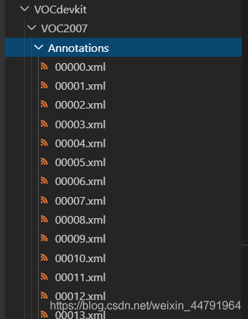
本文使用VOC格式进行训练,训练前需要自己制作好数据集,如果没有自己的数据集,可以通过Github连接下载VOC12+07的数据集尝试下。训练前将标签文件放在VOCdevkit文件夹下的VOC2007文件夹下的Annotation中。
训练前将图片文件放在VOCdevkit文件夹下的VOC2007文件夹下的JPEGImages中。

此时数据集的摆放已经结束。
在完成数据集的摆放之后,我们需要对数据集进行下一步的处理,目的是获得训练用的2007_train.txt以及2007_val.txt,需要用到根目录下的voc_annotation.py。
voc_annotation.py里面有一些参数需要设置。
分别是annotation_mode、classes_path、trainval_percent、train_percent、VOCdevkit_path,第一次训练可以仅修改classes_path
'''
annotation_mode用于指定该文件运行时计算的内容
annotation_mode为0代表整个标签处理过程,包括获得VOCdevkit/VOC2007/ImageSets里面的txt以及训练用的2007_train.txt、2007_val.txt
annotation_mode为1代表获得VOCdevkit/VOC2007/ImageSets里面的txt
annotation_mode为2代表获得训练用的2007_train.txt、2007_val.txt
'''
annotation_mode     = 0
'''
必须要修改,用于生成2007_train.txt、2007_val.txt的目标信息
与训练和预测所用的classes_path一致即可
如果生成的2007_train.txt里面没有目标信息
那么就是因为classes没有设定正确
仅在annotation_mode为0和2的时候有效
'''
classes_path        = 'model_data/voc_classes.txt'
'''
trainval_percent用于指定(训练集+验证集)与测试集的比例,默认情况下 (训练集+验证集):测试集 = 9:1
train_percent用于指定(训练集+验证集)中训练集与验证集的比例,默认情况下 训练集:验证集 = 9:1
仅在annotation_mode为0和1的时候有效
'''
trainval_percent    = 0.9
train_percent       = 0.9
'''
指向VOC数据集所在的文件夹
默认指向根目录下的VOC数据集
'''
VOCdevkit_path  = 'VOCdevkit'
classes_path用于指向检测类别所对应的txt,以voc数据集为例,我们用的txt为:

训练自己的数据集时,可以自己建立一个cls_classes.txt,里面写自己所需要区分的类别。
通过voc_annotation.py我们已经生成了2007_train.txt以及2007_val.txt,此时我们可以开始训练了。
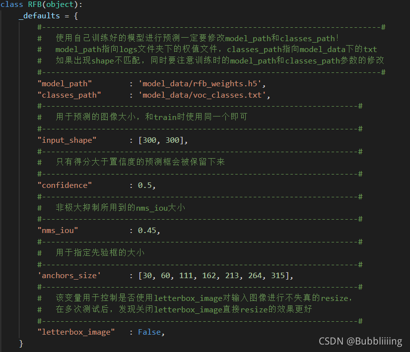
训练的参数较多,大家可以在下载库后仔细看注释,其中最重要的部分依然是train.py里的classes_path。
classes_path用于指向检测类别所对应的txt,这个txt和voc_annotation.py里面的txt一样!训练自己的数据集必须要修改!

修改完classes_path后就可以运行train.py开始训练了,在训练多个epoch后,权值会生成在logs文件夹中。
其它参数的作用如下:
#--------------------------------------------------------#
#   训练前一定要修改classes_path,使其对应自己的数据集
#--------------------------------------------------------#
classes_path    = 'model_data/voc_classes.txt'
#----------------------------------------------------------------------------------------------------------------------------#
#   权值文件请看README,百度网盘下载。数据的预训练权重对不同数据集是通用的,因为特征是通用的。
#   预训练权重对于99%的情况都必须要用,不用的话权值太过随机,特征提取效果不明显,网络训练的结果也不会好。
#   训练自己的数据集时提示维度不匹配正常,预测的东西都不一样了自然维度不匹配
#
#   如果想要断点续练就将model_path设置成logs文件夹下已经训练的权值文件。
#   当model_path = ''的时候不加载整个模型的权值。
#
#   此处使用的是整个模型的权重,因此是在train.py进行加载的。
#   如果想要让模型从主干的预训练权值开始训练,则设置model_path为主干网络的权值,此时仅加载主干。
#   如果想要让模型从0开始训练,则设置model_path = '',Freeze_Train = Fasle,此时从0开始训练,且没有冻结主干的过程。
#   一般来讲,从0开始训练效果会很差,因为权值太过随机,特征提取效果不明显。
#----------------------------------------------------------------------------------------------------------------------------#
model_path      = 'model_data/rfb_weights.h5'
#------------------------------------------------------#
#   输入的shape大小
#------------------------------------------------------#
input_shape     = [300, 300]
#----------------------------------------------------#
#   可用于设定先验框的大小,默认的anchors_size
#   是根据voc数据集设定的,大多数情况下都是通用的!
#   如果想要检测小物体,可以修改anchors_size
#   一般调小浅层先验框的大小就行了!因为浅层负责小物体检测!
#   比如anchors_size = [21, 45, 99, 153, 207, 261, 315]
#----------------------------------------------------#
anchors_size    = [30, 60, 111, 162, 213, 264, 315]
#----------------------------------------------------#
#   训练分为两个阶段,分别是冻结阶段和解冻阶段。
#   显存不足与数据集大小无关,提示显存不足请调小batch_size。
#   受到BatchNorm层影响,batch_size最小为2,不能为1。
#----------------------------------------------------#
#----------------------------------------------------#
#   冻结阶段训练参数
#   此时模型的主干被冻结了,特征提取网络不发生改变
#   占用的显存较小,仅对网络进行微调
#----------------------------------------------------#
Init_Epoch          = 0
Freeze_Epoch        = 50
Freeze_batch_size   = 16
Freeze_lr           = 5e-4
#----------------------------------------------------#
#   解冻阶段训练参数
#   此时模型的主干不被冻结了,特征提取网络会发生改变
#   占用的显存较大,网络所有的参数都会发生改变
#----------------------------------------------------#
UnFreeze_Epoch      = 100
Unfreeze_batch_size = 8
Unfreeze_lr         = 1e-4
#------------------------------------------------------#
#   是否进行冻结训练,默认先冻结主干训练后解冻训练。
#------------------------------------------------------#
Freeze_Train        = True
#------------------------------------------------------#
#   用于设置是否使用多线程读取数据,0代表关闭多线程
#   开启后会加快数据读取速度,但是会占用更多内存
#   keras里开启多线程有些时候速度反而慢了许多
#   在IO为瓶颈的时候再开启多线程,即GPU运算速度远大于读取图片的速度。
#------------------------------------------------------#
num_workers         = 0
#----------------------------------------------------#
#   获得图片路径和标签
#----------------------------------------------------#
train_annotation_path   = '2007_train.txt'
val_annotation_path     = '2007_val.txt'
训练结果预测需要用到两个文件,分别是yolo.py和predict.py。我们首先需要去yolo.py里面修改model_path以及classes_path,这两个参数必须要修改。
model_path指向训练好的权值文件,在logs文件夹里。
classes_path指向检测类别所对应的txt。
完成修改后就可以运行predict.py进行检测了。运行后输入图片路径即可检测。