When it comes to solving classification problems via machine learning, there’s a wide variety of algorithm choices available for almost any data type or niche problem that one might be dealing with. These algorithmic choices can be broadly categorized into two groups, which are as follows.
通过机器学习解决分类问题时,几乎可以处理任何数据类型或细分问题的算法选择很多。 这些算法选择可以大致分为以下两类。
Parametric Algorithms: The algorithms belonging to this category rely on algebraic mathematical equations, that use a set of weights and biases (collectively known as parameters), in order to predict the final discrete outcome for a given set of data. The model size, i.e., the total number of trainable parameters in the model, can vary from just a few (such as, in the case of traditional machine learning algorithms) to millions or even billions (as generally seen in the case of artificial neural nets).
参数算法:属于此类的算法依赖于代数数学方程式,该方程式使用一组权重和偏差(统称为参数),以便预测给定数据集的最终离散结果。 模型的大小,即模型中可训练参数的总数,可以从几个(例如,在传统机器学习算法的情况下)到数百万甚至数十亿(在人工神经网络的情况下通常可以看到)之间变化。网)。
Non-Parametric Algorithms: The classification algorithms in this category are rather unique in the sense that they don’t use any trainable parameters at all. This means that in order to generate predictions, unlike their parametric counterparts, the models in this category don’t rely on a set of weights and biases, or have any assumptions regarding the data. Rather, in order to predict, say, the target class of a new data point, the models use some sort of comparison techniques that help them determine a final outcome.
非参数算法:从根本上讲,它们根本不使用任何可训练的参数,因此该分类算法非常独特。 这意味着,为了生成预测,与其参数对应项不同,此类别中的模型不依赖于一组权重和偏差,也不对数据进行任何假设。 相反,为了预测(例如)新数据点的目标类别,模型使用某种比较技术来帮助他们确定最终结果。
Today, in this article, we are going to study one such non-parametric classification algorithm in detail— the K-Nearest Neighbors (KNN) algorithm.
今天,在本文中,我们将详细研究一种这样的非参数分类算法-K最近邻(KNN)算法。
This is going to be a project-based guide, where in the first part, we will be understanding the basics of the KNN algorithm. This will then be followed by a project where we will be implementing a KNN model from scratch using basic PyData libraries like NumPy and Pandas, while understanding the mathematical foundations of the algorithm.
这将是一个基于项目的指南,在第一部分中,我们将了解KNN算法的基础。 然后是一个项目,在该项目中,我们将使用基本的PyData库(如NumPy和Pandas)从头开始实现KNN模型,同时了解算法的数学基础。
So buckle up, and let’s get started!
系好安全带,让我们开始吧!
KNN分类器基础知识 (KNN Classifier Basics)
To begin with, the KNN algorithm is one of the classic supervised machine learning algorithms that is capable of both binary and multi-class classification. Non-parametric by nature, KNN can also be used as a regression algorithm. However, for the scope of this article, we will only focus on the classification aspect of KNN.
首先,KNN算法是经典的有监督的机器学习算法之一,能够同时进行二进制和多类分类。 KNN本质上是非参数的,也可以用作回归算法。 但是,对于本文的范围,我们仅关注KNN的分类方面。
KNN classification at a glance-
KNN分类一目了然-
→ Supervised algorithm
→监督算法
→ Non-parametric
→非参数
→ Used for both regression and classification
→用于回归和分类
→ Support for both binary and multi-class classification
→支持二进制和多类分类
Before we move any further, let us first break down the definition and understand a few of the terms that we came across.
在继续进行下一步之前,让我们首先分解一下定义并了解我们遇到的一些术语。
KNN is a “supervised” algorithm- In layman's terms, this means that the data used for training a KNN model is a labeled one.
KNN是一种“监督”算法-用外行的话来说,这意味着用于训练KNN模型的数据被标记为一个。
KNN is used for both “binary” and “multi-class classification”- In the machine learning terminology, a classification problem is one where, given a list of discrete values as possible prediction outcomes (known as target classes), the aim of the model is to determine which target class a given data point might belong to. For binary classification problems, the number of possible target classes is 2. On the other hand, a multi-class classification problem, as the name suggests, has more than 2 possible target classes. A KNN classifier can be used to solve either kind of classification problems.
KNN既用于“二进制”分类,也用于“多分类”。在机器学习术语中,分类问题是一种分类问题,其中给定离散值列表作为可能的预测结果(称为目标分类),模型是确定给定数据点可能属于哪个目标类别。 对于二元分类问题,可能的目标类别数目为2。另一方面,顾名思义,多分类问题具有两个以上的可能目标类别。 KNN分类器可用于解决任何一种分类问题。
With that done, we have a rough idea regarding what KNN is. But now, a very important question arises.
完成之后,对于KNN是什么,我们有了一个大概的想法。 但是现在,出现了一个非常重要的问题。
KNN分类器如何工作? (How does a KNN Classifier work?)
As we read earlier, KNN is a non-parametric algorithm. Therefore, training a KNN classifier doesn’t require going through the more traditional approach of iterating over the training data for multiple epochs in order to optimize a set of parameters.
如前所述,KNN是一种非参数算法。 因此,训练KNN分类器不需要经过更传统的方法来迭代多个时期的训练数据以优化一组参数。
Rather, the actual training process in the case of KNN is quite the opposite. Training a KNN model involves simply fitting (or saving) all the training data instances into the computer memory at the same time, which technically requires a single training cycle.
相反,在KNN的情况下,实际的培训过程恰恰相反。 训练KNN模型涉及简单地将所有训练数据实例同时拟合(或保存)到计算机内存中,这在技术上需要一个训练周期。
After this is done, then during the inference stage, where the model has to predict the target class for a completely new data point, the model simply compares this new data with the existing training data instances. Then finally, on the basis of this comparison, the model assigns this new data point to its target class.
完成此操作之后,然后在推理阶段(模型必须为全新的数据点预测目标类别),模型将此新数据与现有训练数据实例进行比较。 最后,在此比较的基础上,模型将该新数据点分配给其目标类。
But now another question arises. What exactly is this comparison that we are talking about, and how does it occur? Well quite honestly, the answer to this question is hidden in the name of the algorithm itself — K-Nearest Neighbors.
但是现在出现了另一个问题。 我们所说的比较到底是什么?它是如何发生的? 坦率地说,这个问题的答案隐藏在算法本身的名称中-K-Nearest Neighbors 。
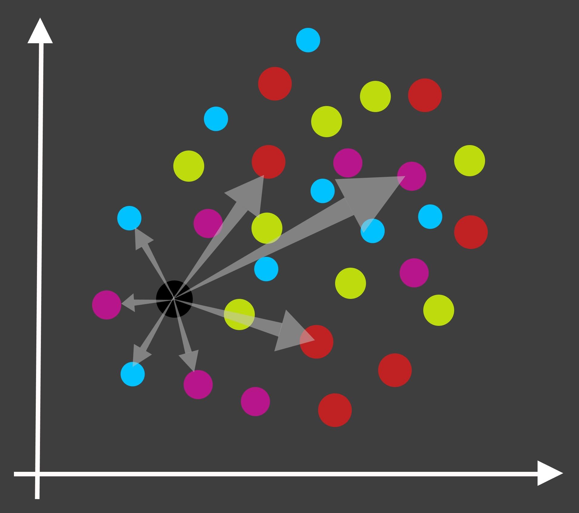
To understand this better, let us dive deeper into how the inference process works.
为了更好地理解这一点,让我们更深入地研究推理过程的工作原理。
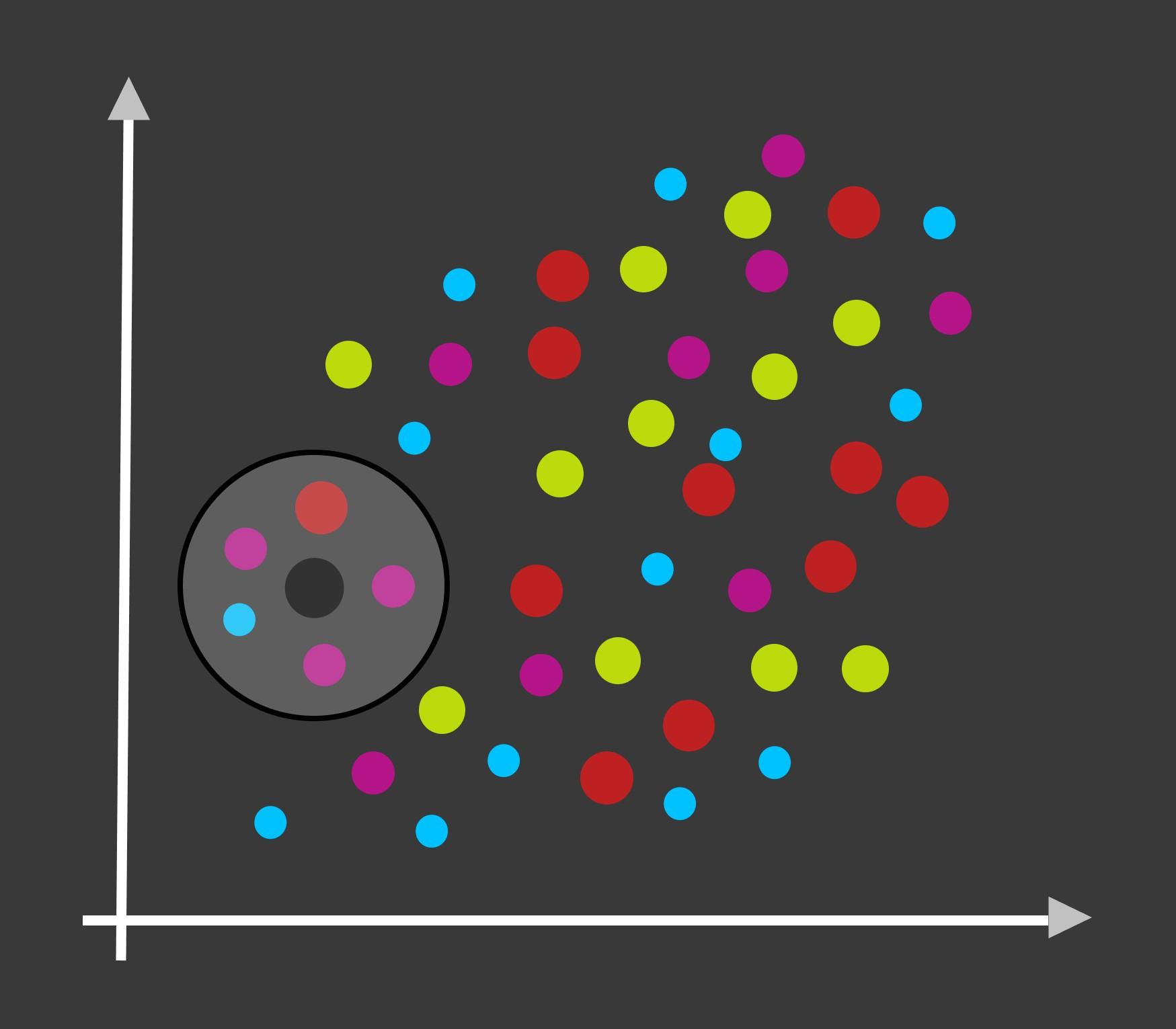
As the first step, our KNN model calculates the distance of this new data point from every single data point within the ‘fitted’ training data.
第一步,我们的KNN模型 计算新数据点与“拟合”训练数据中每个单个数据点的距离。
- Then, in the next step, the algorithm selects ‘k’ number of training data points that are closest to this new data point in terms of the calculated distance. 然后,在下一步中,该算法根据计算出的距离选择最接近此新数据点的'k'个训练数据点。
- Finally, the algorithm compares the target label of these ‘k’ points that are the nearest neighbors to our new data point. The target label with the highest frequency among these k-neighbors is assigned as the target class to the new data point. 最后,算法会比较与新数据点最接近的“ k”个点的目标标签。 在这些k个邻居中频率最高的目标标签被指定为新数据点的目标类别。
And that’s how the KNN classification algorithm works.
这就是KNN分类算法的工作方式。
Regarding the calculation of the distances between the data points, we will be using the Euclidean distance formula. We will be understanding this distance calculation in the next section where we will be code our own KNN-based machine learning model from scratch.
关于数据点之间的距离的计算,我们将使用欧几里得距离公式。 我们将在下一部分中了解距离计算,从头开始编写我们自己的基于KNN的机器学习模型。
So now onto the fun, practical part! We will begin by having a quick glance at the problem statement that we are addressing via our project.
因此,现在进入有趣,实用的部分! 我们将快速浏览一下通过项目解决的问题陈述。
了解问题陈述 (Understanding the Problem Statement)
For this project, we will be working on the famous UCI Red Wine Dataset. The aim of this project is to create a machine learning solution that can predict the quality of a red wine sample.
对于这个项目,我们将研究著名的UCI红酒数据集。 该项目的目的是创建一个可以预测红酒样品质量的机器学习解决方案。
This is a multi-class classification problem. The target variable, i.e., the ‘quality’ of the wine, accepts a discrete integer value ranging from 0–10, where a quality score of 10 denotes a wine of the highest quality standards.
这是一个多类分类问题。 目标变量(即葡萄酒的“质量”)接受介于0到10之间的离散整数值,其中质量得分10表示质量最高的葡萄酒。
Now that we have understood the problem, let us begin with the project by importing all the necessary project dependencies, which includes the necessary PyData modules and the dataset.
既然我们已经了解了问题,那么让我们从导入所有必要的项目依赖项(包括必要的PyData模块和数据集)开始项目。
导入项目依赖项 (Importing Project Dependencies)
In the first step, let us import all the necessary Python modules.
第一步,让我们导入所有必要的Python模块。
Now, let’s import our dataset.
现在,让我们导入数据集。
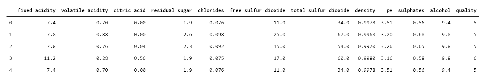
Now that we have imported the dataset, let us try to understand what each of the columns in our data denotes.
现在我们已经导入了数据集,让我们尝试了解数据中每个列的含义。
了解数据 (Understanding the Data)
The following is a brief description of all the individual columns within our dataset.
以下是我们数据集中所有单独列的简要说明。
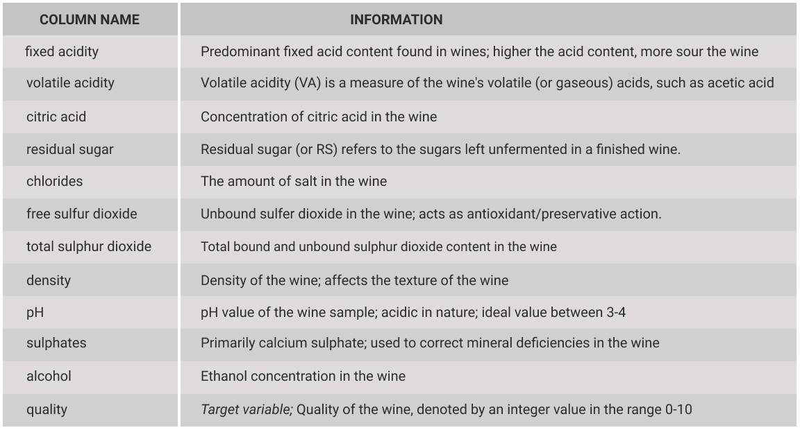
As we discussed earlier, the ‘quality’ column is the target variable for this project. The rest of the columns in the dataset represent the feature variables that will be used for training the model.
正如我们之前讨论的,“质量”列是该项目的目标变量。 数据集中的其余列表示将用于训练模型的特征变量。
Now that we know what the different columns in our dataset represent, let us move on to the next section where we will be doing some pre-processing and exploration of our data.
现在我们知道数据集中的不同列代表什么,让我们继续进行下一部分,在该部分我们将对数据进行一些预处理和探索。
数据整理和EDA (Data Wrangling and EDA)
Data wrangling (or preprocessing) involves analyzing the data to see if it needs any sort of cleaning or scaling so that it can be prepared for training the model.
数据整理(或预处理)涉及分析数据以查看其是否需要任何形式的清理或缩放,以便为训练模型做好准备。
As the first step of data preprocessing, we will check if there are any null values within our data that need to be dealt with.
作为数据预处理的第一步,我们将检查数据中是否有任何空值需要处理。
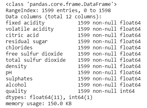
As we can see, there are no null values within our dataset. This is a good thing since we won’t have to deal with any missing data. Now, let us have a look at the statistical analysis of the data.
如我们所见,数据集中没有空值。 这是一件好事,因为我们不必处理任何丢失的数据。 现在,让我们看一下数据的统计分析。
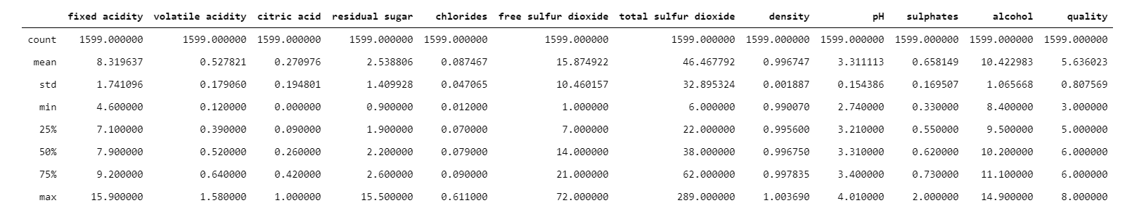
One prominent observation from the above given statistical analysis is that there’s a visible inconsistency in the range of values across different columns within our dataset. To be more clear, the values in some columns are of the order 1e-1 while in a few others, the values can go as high as of the order 1e+2. Because of this inconsistency, there are chances that a feature weight bias might arise at the time of training the model. What is basically means is that some features might end up affecting the final prediction more than the others. Therefore, in order to prevent this weight imbalance, we will have to scale our data.
根据上述统计分析得出的一个突出发现是,我们数据集中不同列之间的值范围存在明显的不一致。 更清楚的是,某些列中的值约为1e-1,而另一些列中的值可能高达1e + 2 。 由于这种不一致,在训练模型时可能会出现特征权重偏差。 基本上,这意味着某些功能可能最终会比其他功能对最终预测的影响更大。 因此,为了防止这种重量失衡,我们将不得不缩放数据。
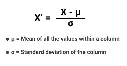
For this scaling, we will be standardizing our data. Standardization typically means rescaling data in a way such that each feature column has a mean of 0 and a standard deviation of 1 (unit variance).
对于这种缩放,我们将对数据进行标准化。 标准化通常意味着以某种方式重新缩放数据,以使每个要素列的平均值为0,标准偏差为1(单位方差)。
The following is the mathematical formula for standard scaling.
以下是用于标准缩放的数学公式。
Now that we know the mathematical formula, let us go ahead and implement this from scratch in Python.
现在我们知道了数学公式,让我们继续在Python中从头开始实现它。
Step-1: Separating the feature matrix and the target array.
步骤1 :分离特征矩阵和目标数组。
Step-2: Declaring the standardization function.
步骤2 :声明标准化功能。
Step-3: Performing standardization on the feature set.
步骤3 :对功能集执行标准化。
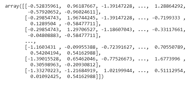
With this, we are done with standardized our data. This will most probably take care of weight bias.
这样,我们就完成了数据标准化。 这很可能会减轻体重。
Now for the last part of our data wrangling and EDA section, we will have a look at the distribution of values across the target column of our dataset.
现在,在数据整理和EDA部分的最后一部分,我们将了解数据集目标列中的值分布。
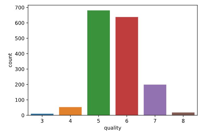
Some of the observations from the above-given graph are-
上图给出的一些观察结果是:
- Most wine samples in our data are rated 5 and 6, followed by 7. 我们数据中的大多数葡萄酒样品的评级为5和6,其次是7。
No wine sample is rated above 8 or below 3. This implies that a wine sample of extremely high quality (9 or 10) or very low quality (0, 1 or 2) rating can either be thought of as a hypothetically ideal situation, or that probably that data is suffering from sampling bias, where the samples of extreme quality didn’t get any representation within the survey.
没有任何葡萄酒样品的评分高于或低于3。这意味着质量极高(9或10)或质量非常低(0、1或2)的葡萄酒样品可以被认为是一种理想的情况,或者这可能是由于样本偏差造成的,即极端质量的样本在调查中没有得到任何代表。
- Our last assumption of a sampling bias within the data is further strengthened as we notice that a majority of wine samples are rated 5 or 6. 由于我们注意到大多数葡萄酒样品的评级为5或6,因此我们对数据中采样偏差的最后一个假设进一步得到了加强。
A model trained on such data will produce biased results, where it is more likely to classify a wine sample as a 5 or 6 on the quality scale as compared to, say, 3 or 8. To know more about sampling bias or how to deal with it, check out this article of mine.
根据此类数据训练的模型会产生偏差的结果,在这种情况下,与3或8相比,更可能将葡萄酒样品按质量等级分类为5或6。要了解更多有关取样偏差或如何处理的信息使用它,查看我的这篇文章。
Now that we are done exploring our data, let us move on to the final part of our project where we will be code our multi-class classifier KNN model using NumPy.
现在,我们已经完成了对数据的探索,让我们继续进行项目的最后部分,在该部分中,我们将使用NumPy对我们的多类分类器KNN模型进行编码。
建模与评估 (Modeling and Evaluation)
As the first step of our modeling process, we will first split our dataset into training and test sets. This is done because training and evaluating your model on the same data is considered a bad practice.
作为建模过程的第一步,我们将首先将数据集分为训练集和测试集。 这样做是因为在相同数据上训练和评估模型被认为是不好的做法。
Let’s see how to implement the code to split the dataset using Python.
让我们看看如何实现使用Python分割数据集的代码。
Step-1: Declaring the split function.
步骤1:声明split函数。
Step-2: Running the splitting function on our standardized dataset.
步骤2:在标准化数据集上运行拆分功能。
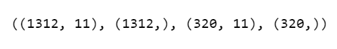
Now that we have created our training and validation sets, we will finally see how to implement the model.
现在,我们已经创建了训练和验证集,我们最终将看到如何实现模型。
On the basis of what we have learned till now, here are the steps involved in creating a KNN model.
根据到目前为止的经验,这里是创建KNN模型的步骤。
Step-1: Training the model- As we read earlier, in the case of KNN, this simply means saving the training dataset within the memory. We have already done that when we created our training and validation data splits.
步骤1:训练模型-正如我们之前所读,对于KNN,这只是意味着将训练数据集保存在内存中。 在创建培训和验证数据拆分时,我们已经做到了。
Step-2: Calculating the distance- A part of the inference process in the KNN algorithm, the process of calculating the distance is an iterative process where we calculate the Euclidean distance of a data point (basically, a data instance/row) in the test data from every single data point within the training data.
步骤2:计算距离-A KNN算法中推理过程的一部分,计算距离的过程是一个迭代过程,在此过程中,我们从测试数据中的每个单个数据点计算数据点(基本上是数据实例/行)的欧几里得距离训练数据。
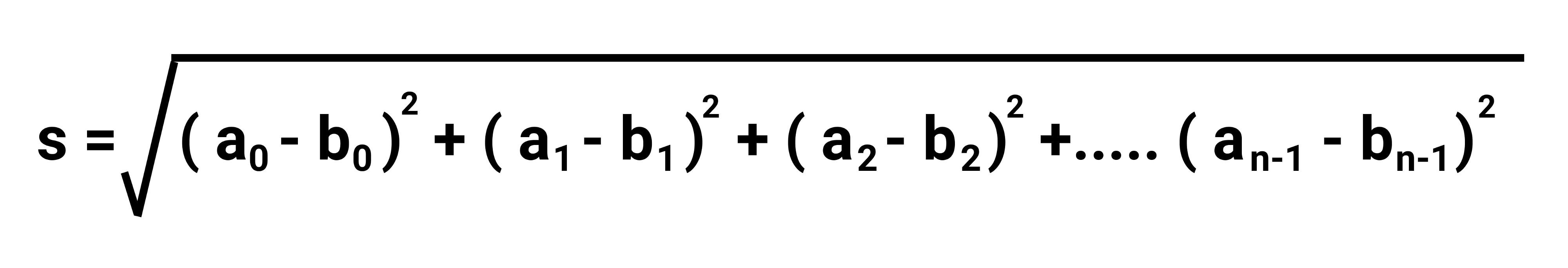
Now, let us understand how the Euclidean distance formula works so that we can implement it for our model.
现在,让我们了解欧几里得距离公式的工作原理,以便可以在模型中实现它。
Let us consider two data points A and B.
让我们考虑两个数据点A和B。
→ A = [a0, a1, a2, a3,…. an], where ai is a feature that represents the data point A.
→A = [A 0,A 1,A 2,A 3,...。 [ n],其中a是代表数据点A的特征。
→ Similarly, B= [b0, b1, b2, b3,…. bn].
→同样, B = [ b 0, b 1 ,b 2 ,b 3 ,…。 b n]。
Therefore, the Euclidean distance between the data points A and B is calculated using the following formula-
因此,数据点A和B之间的欧式距离是使用以下公式计算的:
Let’s now implement this distance calculation step in Python.
现在让我们在Python中实现此距离计算步骤。
Step-2.1: Declaring Python function to calculate Euclidean distance between 2 points.
步骤2.1 :声明Python函数以计算2点之间的欧几里得距离。
Step-2.2: Declaring a Python function to calculate the distance from each point in the training data
步骤2.2 :声明一个Python函数来计算训练数据中每个点的距离
Before we move on to the next step, let us test our distance function.
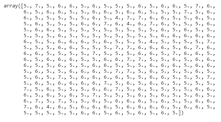
在继续下一步之前,让我们测试距离函数。

As we can see, our distance function successfully calculated the distance of the first point in our test data from all the training data points. Now we can move on to the next step.
如我们所见,我们的距离函数成功地计算出了所有训练数据点中测试数据中第一个点的距离。 现在,我们可以继续下一步。
Step-3: Selecting k-nearest neighbors and making the prediction- This is the final step of the inference stage, where the algorithm selects the k-closest training data points to the test data point based on the distances calculated in step 2. Then, we consider the target labels of these k-nearest neighboring points. The label with the highest occurring frequency is assigned as the target class to the test data point.
步骤3:选择k个最近的邻居并进行预测-这是推理阶段的最后一步,其中算法根据步骤2中计算出的距离,选择距测试数据点最近的k个训练数据点。 ,我们考虑这些k最近邻点的目标标签。 出现频率最高的标签被指定为测试数据点的目标类别。
Let us see how to implement this in Python.
让我们看看如何在Python中实现这一点。
Step-3.1: Defining the KNN Classification function.
步骤3.1 :定义KNN分类功能。
Step-3.2: Running inference on our test dataset.
步骤3.2 :在测试数据集上进行推断。
With this, we have completed the modeling and inference process. As a final step, we will evaluate our models’ performance. For this, we will be using a simple accuracy function that calculates the number of correct predictions made by our model.
至此,我们完成了建模和推理过程。 最后,我们将评估模型的性能。 为此,我们将使用一个简单的精度函数来计算我们的模型做出的正确预测的数量。
Let’s have a look at how to implement the accuracy function in Python.
让我们看一下如何在Python中实现准确性函数。
Step-1: Defining the accuracy function.
步骤1 :定义精度功能。
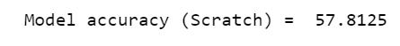
Step-2: Checking the accuracy of our model.
步骤2 :检查模型的准确性。
Step-3: Comparing with the accuracy of a KNN classifier built using the Scikit-Learn library.
步骤3 :与使用Scikit-Learn库构建的KNN分类器的准确性进行比较。
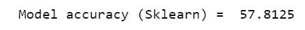
An interesting observation here! Though our model didn’t perform very well (with only 57% correct prediction), it has the exact same accuracy as a Scikit-Learn KNN model. This means the model that we defined from scratch was least able to replicate the performance of a pre-defined model, which is an achievement in itself!
这里有趣的观察! 尽管我们的模型表现不佳(只有57%的正确预测),但其准确性与Scikit-Learn KNN模型完全相同。 这意味着我们从头开始定义的模型最不可能复制预定义模型的性能,这本身就是一项成就!
However, I believe we can further improve the model’s performance to some extent. Therefore, as the last part of our project, we will find the best value of the hyperparameter ‘k’ for which our model gives the highest accuracy.
但是,我相信我们可以在某种程度上进一步改善模型的性能。 因此,作为项目的最后一部分,我们将找到模型为其提供最高准确性的超参数“ k”的最佳值。
模型优化 (Model Optimization)
Before we actually go on to finding the best k-value, first, let us understand the importance of the k-value in the K-Nearest Neighbors algorithm.
在我们继续寻找最佳k值之前,首先,让我们了解k值在K最近邻居算法中的重要性。
- The k-value in the KNN algorithm determines the number of training data points that are to be considered while determining the class of the test data points. KNN算法中的k值确定了确定测试数据点的类别时要考虑的训练数据点的数量。
Impact of a low k-value: If the k-value is very low, say, 1 or 2, the model will become very sensitive to outliers in the data. Outliers can be defined as the extreme instances within the data that do not follow the general trends within the data. Because of this, the predictions of the model become very unstable.
低k值的影响:如果k值非常低,例如1或2,则模型将对数据中的异常值变得非常敏感。 异常值可以定义为数据中的极端实例,这些极端实例不遵循数据中的总体趋势。 因此,模型的预测变得非常不稳定。
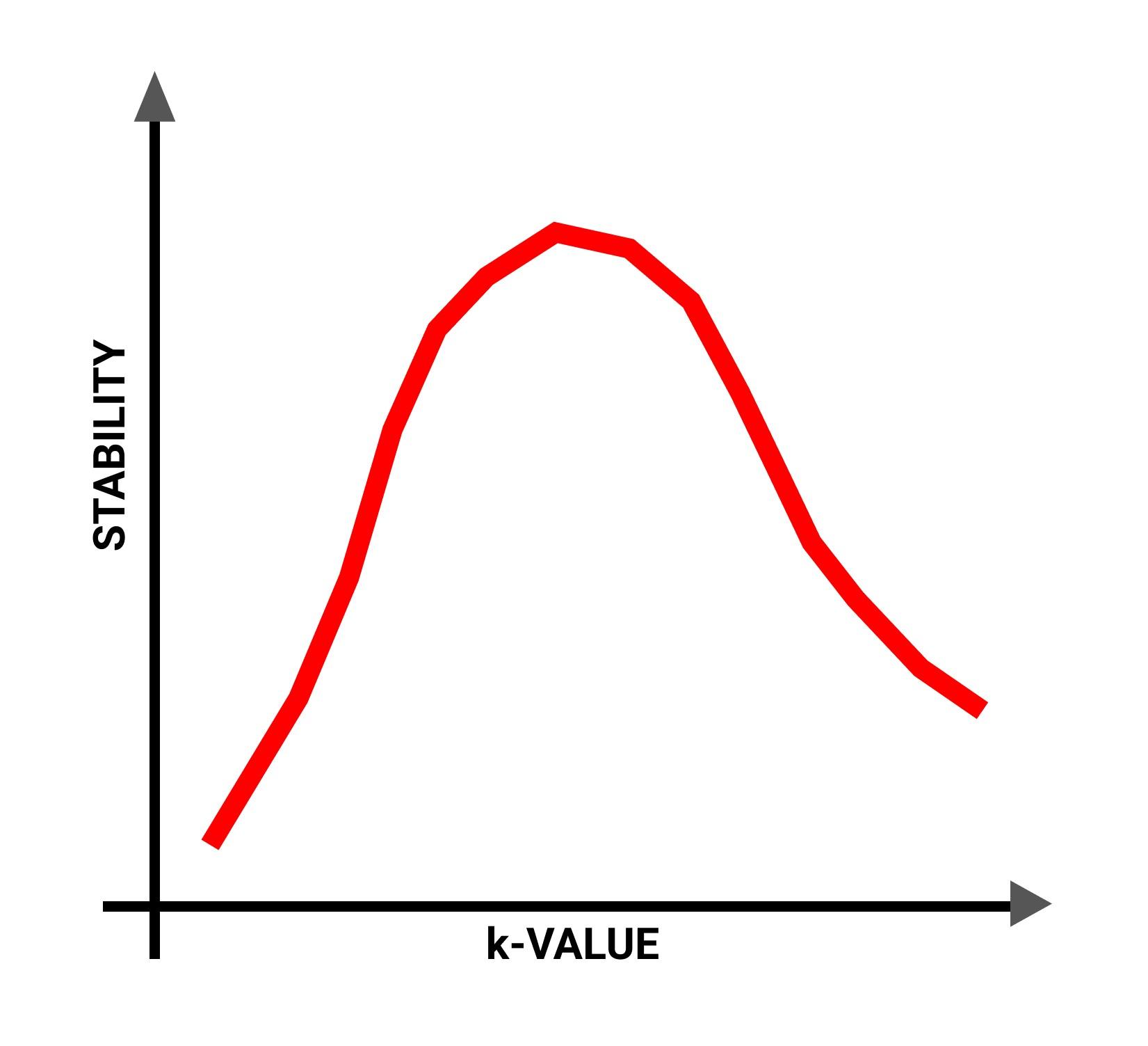
Impact of a high k-value: Now, as the k-value in the KNN algorithm increases, a weird trend is observed. At first, an increase is observed in the stability of the algorithm. One reason for this can be that as we consider more neighbors for predicting the target class of a test data point, because of majority voting, the effect of outliers decreases. However, as we continue to increase the k-value, after a certain point, we start to observe a decline in the stability of the algorithm, and the model accuracy starts to deteriorate.
高k值的影响:现在,随着KNN算法中k值的增加,观察到一个奇怪的趋势。 首先,观察到算法稳定性的增加。 原因之一可能是,由于我们考虑使用更多的邻居来预测测试数据点的目标类别,因此由于多数表决,离群值的影响减小了。 但是,随着我们继续增加k值,在某个点之后,我们开始观察到算法稳定性的下降,并且模型准确性开始下降。
The following graph roughly represents the relation between the k-value and stability of a KNN classifier model.
下图大致表示K值分类器模型的k值与稳定性之间的关系。
Now, let us finally evaluate the model for a range of different k-values. The one with the highest accuracy will be chosen as the final k-value for our model.
现在,让我们最终评估模型的一系列不同k值。 精度最高的模型将被选为模型的最终k值。
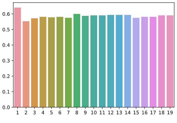
As we can see, k-value 1 has the highest accuracy. But as we discussed earlier, for k=1, the model will be very sensitive to outliers. Hence, we will go with k=8 which has the second-highest accuracy. Let us observe the results with k=8.
如我们所见,k值1的准确性最高。 但是正如我们前面讨论的,对于k = 1,该模型对异常值非常敏感。 因此,我们将使用k = 8,它具有第二高的精度。 让我们观察k = 8的结果。
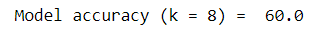
As you can see, we got a performance boost here! Just by tweaking the hyperparameter ‘k’, our model’s accuracy bumped up by almost 3 percent.
如您所见,我们在这里获得了性能提升! 仅通过调整超参数“ k”,我们模型的精度就提高了近3%。
With this, we come to the end of our project.
这样,我们就结束了我们的项目。
To finish things off, let us have a quick rundown of all that we learned today, as well as some of the key takeaways from this lesson.
最后,让我们快速总结一下我们今天所学到的所有知识,以及本课中的一些重要内容。
结论 (Conclusions)
In this article, we had an in-depth analysis of the K-Nearest Neighbors classification algorithm. We understood how the algorithm uses Euclidean distance between the data instances as a criterion of comparison, on the basis of which it predicts the target class for a particular data instance.
在本文中,我们对K最近邻居分类算法进行了深入分析。 我们了解了该算法如何使用数据实例之间的欧式距离作为比较标准,并以此为基础预测特定数据实例的目标类别。
In the second part of this guide, we went through a step-by-step process of creating a KNN classification model from scratch, primarily using Python and NumPy.
在本指南的第二部分中,我们逐步进行了从头开始创建KNN分类模型的逐步过程,主要使用Python和NumPy。
Though our model was not able to give a stellar performance, at least we were able to match the performance of a predefined Scikit-Learn mode. Now, while we were able to increase the model’s accuracy up to 60% via hyperparameter optimization, the performance was still not apt.
尽管我们的模型无法提供出色的性能,但至少我们能够匹配预定义的Scikit-Learn模式的性能。 现在,尽管我们可以通过超参数优化将模型的精度提高到60%,但性能仍然不合适。
This has a lot to do with how the data was structured. As we observed earlier, there was a huge sampling bias in the data. This certainly affected our model’s performance. Another reason for the poor performance can be that probably, the data had a large number of outliers. All this brings us to a very important part that I left for the very end, where we will have a look at the advantages and disadvantages of the KNN classification algorithm.
这与数据的结构有很大关系。 正如我们之前观察到的,数据中存在巨大的采样偏差。 这无疑影响了我们模型的性能。 性能不佳的另一个原因可能是数据中有大量异常值。 所有这些将我们带到了我最后要提到的非常重要的部分,在这里我们将了解KNN分类算法的优缺点。
KNN-的优势 (Advantages of KNN-)
As we discussed earlier, being a non-parametric algorithm, KNN doesn’t require multiple training cycles in order to adapt to the trends within the training data. As a result of this, KNN has an almost negligible training time, and in fact, is one of the fastest machine learning algorithms when it comes to training.
如前所述,作为一种非参数算法,KNN不需要多个训练周期即可适应训练数据中的趋势。 因此,KNN的训练时间几乎可以忽略不计,实际上,它是训练时最快的机器学习算法之一。
The implementation of KNN is very easy, as compared to some other, more complex classification algorithms.
与其他一些更复杂的分类算法相比,KNN的实现非常容易。
KNN的缺点 (Disadvantages of KNN–)
When it comes to inference, KNN is very compute-intensive. For inference on each test data instance, the algorithm has to calculate its distance from every single point in the training data. In terms of time complexity, for n-number of training data instances and m-number of test data instances, the complexity of the algorithm evaluates to O(m x n).
说到推理,KNN的计算量很大。 为了推断每个测试数据实例,算法必须计算其与训练数据中每个点的距离。 就时间复杂度而言,对于n个训练数据实例和m个测试数据实例,算法的复杂度评估为O(mxn) 。
As the dimensionality (i.e., the total number of features) and the scale of the dataset (i.e., the total number of data instances) increases, the model size also increases, which in turn impacts the performance and speed of the model. Therefore, KNN is not a good algorithm choice when it comes to high dimensional, large scale datasets.
随着维度(即要素的总数)和数据集的规模(即数据实例的总数)的增加,模型的大小也随之增加,进而影响模型的性能和速度。 因此,对于高维,大规模数据集,KNN并不是一个好的算法选择。
The KNN algorithm is very sensitive to outliers in the data. Even a slight increase in the noise within the dataset might drastically affect the model’s performance.
KNN算法对数据中的异常值非常敏感。 即使数据集中的噪声稍微增加,也可能严重影响模型的性能。
With this, we finally come to an end of today’s learning session. In another article of mine, I have directly pitted a bunch of machine learning algorithms against each other. There, you can check out how KNN fares against other classification algorithms like logistic regression, decision tree classifiers, random forest ensembles, etc.
这样,我们终于结束了今天的学习环节。 在我的另一篇文章中,我直接将一堆机器学习算法相互比较。 在那里,您可以查看KNN如何与其他分类算法(例如逻辑回归,决策树分类器,随机森林合奏等)相提并论。
By the way, this was the fourth article in my ML from Scratch series, where I cover different machine learning algorithms and their mathematical foundations in detail. If you are interested in learning more, the other articles in this series are-
顺便说一句,这是我的Scratch系列机器学习中的第四篇文章,其中我详细介绍了不同的机器学习算法及其数学基础。 如果您有兴趣了解更多信息,本系列的其他文章是-
Link to the project GitHub files.
If you liked the article and would love to keep seeing more articles in the ML from Scratch series, make sure you hit that follow button.
如果您喜欢这篇文章并且希望继续在Scratch系列的ML中看到更多文章,请确保单击该关注按钮。
Happy learning!
学习愉快!
翻译自: https://towardsdatascience.com/ml-from-scratch-k-nearest-neighbors-classifier-3fc51438346b